Quickstart
This page shows how to use the package on a simulated example. We first generate panel data, inspect its basic evolution, then estimate the cohort-time \(LATT(e, t)\) parameters, and finally aggregate them into event-study effects. We also show how to specify a DML estimator in DML. The repeated cross-sections case has the exact same syntax; only the simulated data differs.
Installation
Install the package from PyPI with:
uv pip install idid-py
or from Github
uv pip install git+https://github.com/jsr-p/idid
or install the local development version with:
git clone https://github.com/jsr-p/idid && cd idid
uv sync
Panel data
Data
 1import numpy as np
 2import polars as pl
 3
 4import idid
 5
 6np.random.seed(40)
 7n = 10_000
 8E_cohorts = [0, 2, 3, 4, 5]
 9T = max(E_cohorts)
10
11data = idid.sim_stag_panel(n=n, T=T, E_cohorts=E_cohorts)
12
13with pl.Config(tbl_rows=10, tbl_cols=10):
14    print(data.head(10))
shape: (10, 6)
┌─────┬─────┬─────┬───────────┬─────┬───────────┐
│ id  ┆ E   ┆ t   ┆ X         ┆ D_t ┆ Y_t       │
│ --- ┆ --- ┆ --- ┆ ---       ┆ --- ┆ ---       │
│ i64 ┆ i64 ┆ i64 ┆ f64       ┆ i64 ┆ f64       │
╞═════╪═════╪═════╪═══════════╪═════╪═══════════╡
│ 0   ┆ 0   ┆ 1   ┆ -0.607548 ┆ 0   ┆ -0.682584 │
│ 0   ┆ 0   ┆ 2   ┆ -0.607548 ┆ 0   ┆ 0.089033  │
│ 0   ┆ 0   ┆ 3   ┆ -0.607548 ┆ 1   ┆ 3.061392  │
│ 0   ┆ 0   ┆ 4   ┆ -0.607548 ┆ 0   ┆ 0.186256  │
│ 0   ┆ 0   ┆ 5   ┆ -0.607548 ┆ 0   ┆ -0.989965 │
│ 1   ┆ 0   ┆ 1   ┆ -0.126136 ┆ 0   ┆ -0.09219  │
│ 1   ┆ 0   ┆ 2   ┆ -0.126136 ┆ 0   ┆ -0.620078 │
│ 1   ┆ 0   ┆ 3   ┆ -0.126136 ┆ 0   ┆ -1.533602 │
│ 1   ┆ 0   ┆ 4   ┆ -0.126136 ┆ 0   ┆ -0.117459 │
│ 1   ┆ 0   ┆ 5   ┆ -0.126136 ┆ 0   ┆ 1.390381  │
└─────┴─────┴─────┴───────────┴─────┴───────────┘
Plotting the evolution of the treatment and outcome gives:
1from idid.plotting import plot_evolution, summarize_evolution
2
3fig, ax = plot_evolution(
4    summarize_evolution(data),
5    include_bands=True,
6)
7fig
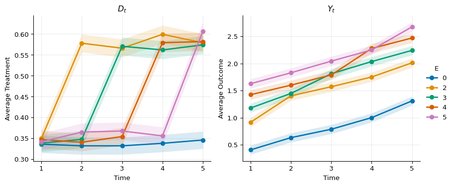
The true simulated effects are \(LATT(e, t) = 1\) for all \(e \geq t\).
Estimating all LATT(e, t)s
 1res = idid.estimate(
 2    data,
 3    cohort="E",
 4    time="t",
 5    outcome="Y_t",
 6    treatment="D_t",
 7    unit="id",
 8    covariates=["X"],
 9    control="never",
10    method="dr",
11    balanced=True,
12    verbose=False,
13)
14print(res)
IDidResult(n=10000, dp=IDidParams(e_col='E', t_col='t', d_col='D_t', y_col='Y_t'), periods=Periods(...), estimates=DataFrame[10x9; E, t, latt, se, ...], IFs=ndarray(10000, 10), IFs_aet=ndarray(10000, 10))
We can inspect the estimates as a DataFrame:
1with pl.Config(tbl_rows=10, tbl_cols=10):
2  print(res.estimates)
shape: (10, 9)
┌─────┬─────┬──────────┬──────────┬──────────┬──────────┬──────┬──────────┬──────────┐
│ E   ┆ t   ┆ latt     ┆ se       ┆ num      ┆ denom    ┆ ns   ┆ lower    ┆ upper    │
│ --- ┆ --- ┆ ---      ┆ ---      ┆ ---      ┆ ---      ┆ ---  ┆ ---      ┆ ---      │
│ i64 ┆ i64 ┆ f64      ┆ f64      ┆ f64      ┆ f64      ┆ i64  ┆ f64      ┆ f64      │
╞═════╪═════╪══════════╪══════════╪══════════╪══════════╪══════╪══════════╪══════════╡
│ 2   ┆ 2   ┆ 1.115836 ┆ 0.230915 ┆ 0.258145 ┆ 0.231346 ┆ 4022 ┆ 0.663243 ┆ 1.568428 │
│ 2   ┆ 3   ┆ 1.225298 ┆ 0.244773 ┆ 0.268993 ┆ 0.219533 ┆ 4022 ┆ 0.745543 ┆ 1.705053 │
│ 2   ┆ 4   ┆ 0.966331 ┆ 0.216551 ┆ 0.237252 ┆ 0.245519 ┆ 4022 ┆ 0.541892 ┆ 1.39077  │
│ 2   ┆ 5   ┆ 0.86206  ┆ 0.24246  ┆ 0.188788 ┆ 0.218997 ┆ 4022 ┆ 0.386838 ┆ 1.337281 │
│ 3   ┆ 3   ┆ 0.91629  ┆ 0.234961 ┆ 0.20478  ┆ 0.223488 ┆ 4046 ┆ 0.455767 ┆ 1.376814 │
│ 3   ┆ 4   ┆ 1.062971 ┆ 0.258129 ┆ 0.21958  ┆ 0.206572 ┆ 4046 ┆ 0.557037 ┆ 1.568904 │
│ 3   ┆ 5   ┆ 0.535162 ┆ 0.251652 ┆ 0.114376 ┆ 0.213722 ┆ 4046 ┆ 0.041925 ┆ 1.028399 │
│ 4   ┆ 4   ┆ 1.288046 ┆ 0.248529 ┆ 0.27902  ┆ 0.216622 ┆ 3976 ┆ 0.800929 ┆ 1.775164 │
│ 4   ┆ 5   ┆ 0.749072 ┆ 0.248445 ┆ 0.16084  ┆ 0.214718 ┆ 3976 ┆ 0.26212  ┆ 1.236023 │
│ 5   ┆ 5   ┆ 0.461413 ┆ 0.223437 ┆ 0.114358 ┆ 0.247844 ┆ 3995 ┆ 0.023476 ┆ 0.899349 │
└─────┴─────┴──────────┴──────────┴──────────┴──────────┴──────┴──────────┴──────────┘
or print out a summary:
1res.summary()
Cohort-Time Local Average Treatment Effects on the Treated:
 E   t    AET(e, t)   LATT(e, t)   Std. Error   [95% Pointwise.   Conf. Band]
 2   2       0.2313       1.1158       0.2309            0.6632        1.5684  *
 2   3       0.2195       1.2253       0.2448            0.7455        1.7051  *
 2   4       0.2455       0.9663       0.2166            0.5419        1.3908  *
 2   5       0.2190       0.8621       0.2425            0.3868        1.3373  *
 3   3       0.2235       0.9163       0.2350            0.4558        1.3768  *
 3   4       0.2066       1.0630       0.2581            0.5570        1.5689  *
 3   5       0.2137       0.5352       0.2517            0.0419        1.0284  *
 4   4       0.2166       1.2880       0.2485            0.8009        1.7752  *
 4   5       0.2147       0.7491       0.2484            0.2621        1.2360  *
 5   5       0.2478       0.4614       0.2234            0.0235        0.8993  *
---
Signif. codes: `*' confidence band does not cover 0
Control group: Never treated
Estimation Method: Doubly Robust
The IDidResult result object is documented in
IDidResult.
Aggregated Effects
1agg = idid.agg_latt(res, method="dynamic")
2print(agg)
AggLattResult(method='dynamic', overall_latt=0.893323526028491, overall_se=0.1249504706156244, estimates=DataFrame[4x5; l, latt, se, lower, ...], IF=ndarray(10000, 4), IF_overall=ndarray(10000, 1))
These correspond to estimates of the \(\{\theta^{IV}_{es}(l) : l \in \{0,1,\ldots,h\}\}\) parameters of the paper.
Again, we can inspect the estimates as a DataFrame:
1print(agg.estimates)
shape: (4, 5)
┌─────┬──────────┬──────────┬──────────┬──────────┐
│ l   ┆ latt     ┆ se       ┆ lower    ┆ upper    │
│ --- ┆ ---      ┆ ---      ┆ ---      ┆ ---      │
│ i64 ┆ f64      ┆ f64      ┆ f64      ┆ f64      │
╞═════╪══════════╪══════════╪══════════╪══════════╡
│ 0   ┆ 0.931205 ┆ 0.091954 ┆ 0.750976 ┆ 1.111434 │
│ 1   ┆ 1.015631 ┆ 0.13086  ┆ 0.759145 ┆ 1.272117 │
│ 2   ┆ 0.764398 ┆ 0.162559 ┆ 0.445783 ┆ 1.083013 │
│ 3   ┆ 0.86206  ┆ 0.24246  ┆ 0.386838 ┆ 1.337281 │
└─────┴──────────┴──────────┴──────────┴──────────┘
or print out a summary:
1agg.summary()
Overall summary of ATT's based on event-study/dynamic aggregation:
  LATT    Std. Error    [95%      Conf. Band]
0.8933        0.1250    0.6484         1.1382  *

Dynamic effects:
  Event time    Estimate    Std. Error    [95% Pointwise    Conf. Band]
           0      0.9312        0.0920            0.7510         1.1114  *
           1      1.0156        0.1309            0.7591         1.2721  *
           2      0.7644        0.1626            0.4458         1.0830  *
           3      0.8621        0.2425            0.3868         1.3373  *
---
Signif. codes: `*' confidence band does not cover 0
Control group: Never treated
Estimation Method: Doubly Robust
The AggLattResult result object is documented in
AggLattResult. See also
extended guide in Aggregation.
Multiplier Bootstrap and Simultaneous Confidence Bands
We can conduct multiplier bootstrap to obtain simultaneous confidence bands on all the event study parameters:
1agg_b = idid.agg_latt(res, method="dynamic", boot=True)
2agg_b.summary()
Overall summary of ATT's based on event-study/dynamic aggregation:
  LATT    Std. Error    [95% Simult.    Conf. Band]
0.8933        0.1246          0.6448         1.1419  *

Dynamic effects:
  Event time    Estimate    Std. Error    [95% Simult.    Conf. Band]
           0      0.9312        0.0926          0.7036         1.1588  *
           1      1.0156        0.1302          0.6956         1.3356  *
           2      0.7644        0.1640          0.3614         1.1674  *
           3      0.8621        0.2337          0.2876         1.4366  *
---
Signif. codes: `*' confidence band does not cover 0
Control group: Never treated
Estimation Method: Doubly Robust
Multiplier bootstrap: B=1000, c=2.4580, overall c=1.9942
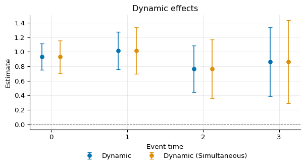
Comparing the two in a figure:
 1from idid.plotting import plot_agg
 2from matplotlib import pyplot as plt
 3
 4fig, ax = plot_agg(
 5    [agg, agg_b],
 6    labels=[
 7        "Dynamic",
 8        "Dynamic (Simultaneous)",
 9    ],
10)
DML
Using linear regression for the outcome nuisance model and FastLogit
for the treatment nuisance models:
 1from idid.nuisance_estimators import OLS, FastLogit
 2
 3
 4res_dml = idid.estimate(
 5    data,
 6    cohort="E",
 7    time="t",
 8    outcome="Y_t",
 9    treatment="D_t",
10    unit="id",
11    covariates=["X"],
12    control="never",
13    method="dml",
14    dml_kwargs={
15        "nfolds": 5,
16        "m_m": OLS(),
17        "g_m": FastLogit(),
18        "p_m": FastLogit(),
19    },
20    balanced=True,
21    verbose=False,
22)
23
24res_dml.summary()
Cohort-Time Local Average Treatment Effects on the Treated:
 E   t    AET(e, t)   LATT(e, t)   Std. Error   [95% Pointwise.   Conf. Band]
 2   2       0.2311       1.1174       0.2313            0.6641        1.5707  *
 2   3       0.2190       1.2323       0.2456            0.7510        1.7137  *
 2   4       0.2453       0.9707       0.2169            0.5455        1.3959  *
 2   5       0.2187       0.8720       0.2431            0.3955        1.3485  *
 3   3       0.2237       0.9163       0.2348            0.4561        1.3766  *
 3   4       0.2073       1.0554       0.2573            0.5510        1.5598  *
 3   5       0.2139       0.5332       0.2517            0.0399        1.0265  *
 4   4       0.2166       1.2848       0.2487            0.7973        1.7723  *
 4   5       0.2141       0.7480       0.2495            0.2590        1.2370  *
 5   5       0.2474       0.4659       0.2236            0.0276        0.9041  *
---
Signif. codes: `*' confidence band does not cover 0
Control group: Never treated
Estimation Method: Double Machine Learning
DML nuisance models: m_m=OLS, g_m=FastLogit, p_m=FastLogit
DML cross-fitting folds: 5
FastLogit comes from
fastlr.
Using sklearn objects for the nuisance models:
 1from sklearn.linear_model import LinearRegression, LogisticRegression
 2
 3
 4res_dml_sk = idid.estimate(
 5    data,
 6    cohort="E",
 7    time="t",
 8    outcome="Y_t",
 9    treatment="D_t",
10    unit="id",
11    covariates=["X"],
12    control="never",
13    method="dml",
14    dml_kwargs={
15        "nfolds": 5,
16        "m_m": LinearRegression(),
17        "g_m": LogisticRegression(),
18        "p_m": LogisticRegression(),
19    },
20    balanced=True,
21    verbose=False,
22)
23
24res_dml_sk.summary()
Cohort-Time Local Average Treatment Effects on the Treated:
 E   t    AET(e, t)   LATT(e, t)   Std. Error   [95% Pointwise.   Conf. Band]
 2   2       0.2311       1.1174       0.2313            0.6641        1.5707  *
 2   3       0.2190       1.2323       0.2456            0.7510        1.7137  *
 2   4       0.2453       0.9707       0.2169            0.5455        1.3959  *
 2   5       0.2187       0.8720       0.2431            0.3955        1.3485  *
 3   3       0.2237       0.9163       0.2348            0.4561        1.3765  *
 3   4       0.2072       1.0554       0.2573            0.5510        1.5598  *
 3   5       0.2139       0.5332       0.2517            0.0399        1.0265  *
 4   4       0.2166       1.2848       0.2487            0.7974        1.7723  *
 4   5       0.2141       0.7480       0.2495            0.2590        1.2370  *
 5   5       0.2474       0.4659       0.2236            0.0277        0.9041  *
---
Signif. codes: `*' confidence band does not cover 0
Control group: Never treated
Estimation Method: Double Machine Learning
DML nuisance models: m_m=LinearRegression, g_m=LogisticRegression, p_m=LogisticRegression
DML cross-fitting folds: 5
The dml_kwargs argument is documented in
DMLKwargs.
Repeated cross-sections
The repeated cross-section case is handled analogously to the panel
case; the only difference is setting balanced=False in the estimate
function.
 1import numpy as np
 2import polars as pl
 3
 4import idid
 5
 6np.random.seed(40)
 7n = 10_000
 8E_cohorts = [0, 2, 3, 4, 5]
 9T = max(E_cohorts)
10
11data = idid.sim_stag_rc(n=n, T=T, E_cohorts=E_cohorts)
12
13with pl.Config(tbl_rows=10, tbl_cols=10):
14    print(data.head(10))
shape: (10, 6)
┌─────┬─────┬─────┬───────────┬─────┬───────────┐
│ id  ┆ E   ┆ t   ┆ X         ┆ D_t ┆ Y_t       │
│ --- ┆ --- ┆ --- ┆ ---       ┆ --- ┆ ---       │
│ u32 ┆ i64 ┆ i64 ┆ f64       ┆ i64 ┆ f64       │
╞═════╪═════╪═════╪═══════════╪═════╪═══════════╡
│ 1   ┆ 5   ┆ 1   ┆ -0.607548 ┆ 0   ┆ 0.01554   │
│ 2   ┆ 3   ┆ 2   ┆ 0.545059  ┆ 1   ┆ 0.92165   │
│ 3   ┆ 5   ┆ 3   ┆ 0.188836  ┆ 0   ┆ 1.154266  │
│ 4   ┆ 0   ┆ 4   ┆ -0.982146 ┆ 0   ┆ 0.417061  │
│ 5   ┆ 5   ┆ 5   ┆ 0.639967  ┆ 1   ┆ 3.541751  │
│ 6   ┆ 3   ┆ 1   ┆ 0.842739  ┆ 0   ┆ 2.511837  │
│ 7   ┆ 2   ┆ 2   ┆ -0.604616 ┆ 1   ┆ 1.386531  │
│ 8   ┆ 0   ┆ 3   ┆ -0.770702 ┆ 0   ┆ -1.107861 │
│ 9   ┆ 4   ┆ 4   ┆ 1.446865  ┆ 1   ┆ 4.404883  │
│ 10  ┆ 5   ┆ 5   ┆ 1.991825  ┆ 1   ┆ 2.465375  │
└─────┴─────┴─────┴───────────┴─────┴───────────┘
 1res = idid.estimate(
 2    data,
 3    cohort="E",
 4    time="t",
 5    outcome="Y_t",
 6    treatment="D_t",
 7    unit="id",
 8    covariates=["X"],
 9    control="never",
10    method="dr",
11    balanced=False,
12    verbose=False,
13)
14res.summary()
Cohort-Time Local Average Treatment Effects on the Treated:
 E   t    AET(e, t)   LATT(e, t)   Std. Error   [95% Pointwise.   Conf. Band]
 2   2       0.2438       2.2645       0.6899            0.9124        3.6166  *
 2   3       0.1709       2.6230       0.9937            0.6753        4.5707  *
 2   4       0.1572       2.3952       1.0712            0.2957        4.4947  *
 2   5       0.2008       2.0019       0.8194            0.3959        3.6079  *
 3   3       0.1715       1.0047       0.9070           -0.7730        2.7824
 3   4       0.1882       1.2923       0.8183           -0.3116        2.8962
 3   5       0.2526       1.9867       0.6433            0.7259        3.2475  *
 4   4       0.2911       0.9887       0.5361           -0.0621        2.0394
 4   5       0.3185       1.0436       0.4999            0.0638        2.0234  *
 5   5       0.2761       1.7817       0.5973            0.6109        2.9525  *
---
Signif. codes: `*' confidence band does not cover 0
Control group: Never treated
Estimation Method: Doubly Robust
1agg = idid.agg_latt(res, method="dynamic")
2print(agg.estimates)
shape: (4, 5)
┌─────┬──────────┬──────────┬──────────┬──────────┐
│ l   ┆ latt     ┆ se       ┆ lower    ┆ upper    │
│ --- ┆ ---      ┆ ---      ┆ ---      ┆ ---      │
│ i64 ┆ f64      ┆ f64      ┆ f64      ┆ f64      │
╞═════╪══════════╪══════════╪══════════╪══════════╡
│ 0   ┆ 1.538493 ┆ 0.262079 ┆ 1.024819 ┆ 2.052167 │
│ 1   ┆ 1.521017 ┆ 0.369766 ┆ 0.796275 ┆ 2.245759 │
│ 2   ┆ 2.144508 ┆ 0.568804 ┆ 1.029653 ┆ 3.259363 │
│ 3   ┆ 2.001893 ┆ 0.819383 ┆ 0.395903 ┆ 3.607884 │
└─────┴──────────┴──────────┴──────────┴──────────┘