Aggregation

Aggregation Methods

This page shows how the package aggregates estimated cohort-time \(LATT(e,t)\)s into the main summary measures used in the paper: event-study effects by horizon, balanced event-study effects, cohort-specific effects, calendar-time effects, cumulative calendar-time effects, and overall effects.

import idid

data = idid.sim_stag_panel(n=10_000, T=5, E_cohorts=[0, 2, 3, 4, 5])
res = idid.estimate(
    data,
    cohort="E",
    time="t",
    outcome="Y_t",
    treatment="D_t",
    unit="id",
    covariates=["X"],
    control="never",
    method="dr",
    balanced=True,
    verbose=False,
)
dynamic = idid.agg_latt(res, method="dynamic")
dynamic.summary()

Overall summary of ATT's based on event-study/dynamic aggregation:
  LATT    Std. Error    [95%      Conf. Band]
1.0047        0.1281    0.7537         1.2557  *

Dynamic effects:
  Event time    Estimate    Std. Error    [95% Pointwise    Conf. Band]
           0      0.8868        0.0946            0.7013         1.0723  *
           1      0.9157        0.1215            0.6775         1.1539  *
           2      0.8853        0.1631            0.5656         1.2051  *
           3      1.3310        0.2582            0.8249         1.8371  *
---
Signif. codes: `*' confidence band does not cover 0
Control group: Never treated
Estimation Method: Doubly Robust

The method argument accepts AggMethod.

Method	Description
"dynamic"	aggregate by event-time horizon l := t - E
"dynamic_bal"	balanced event-time aggregation
"cohort"	aggregate by exposure cohort
"group"	alias for cohort aggregation
"calendar"	aggregate by calendar time
"calendar_cumu"	cumulative calendar-time aggregation
"simple"	aggregate all post-exposure LATTs

Weighted Estimands

The general weighted estimand has the form:

\[ \theta = \sum_{e \in \mathcal{E}} \sum_{t = 2}^{\mathcal{T}} w(e,t)\, LATT(e,t),\]

where \(w(e,t)\) denotes a weighting scheme.

The figure below is the overview of the different weighted estimands and their weights from the paper:

The corresponding idid.agg_latt(..., method=...) mappings for the complier-weighted IDiD aggregations are:

Paper parameter	Code
\(\theta^{IV}_{es}(l)\)	"dynamic"
\(\theta^{IV}_{bal,es}(l,l')\)	"dynamic_bal"
\(\theta^{IV}_{sel}(\tilde{e})\)	"cohort" or "group"
\(\theta^{IV}_{c}(\tilde{t})\)	"calendar"
\(\theta^{cumm,IV}_{c}(\tilde{t})\)	"calendar_cumu"
\(\theta^{o,IV}_{W}\)	"simple"
\(\theta^{o,IV}_{sel}\)	overall summary reported by "cohort" / "group"

When complier_weighted=False, agg_latt switches to the CSA-style aggregations corresponding to the lower row of the figure:

Paper parameter	Code
\(\theta_{es}(l)\)	method="dynamic", complier_weighted=False
\(\theta_{bal,es}(l,l')\)	method="dynamic_bal", complier_weighted=False
\(\theta_{sel}(\tilde{e})\)	method="cohort" or "group", complier_weighted=False
\(\theta_{c}(\tilde{t})\)	method="calendar", complier_weighted=False
\(\theta^{cumm}_{c}(\tilde{t})\)	method="calendar_cumu", complier_weighted=False
\(\theta^{o}_{W}\)	method="simple", complier_weighted=False
\(\theta^{o}_{sel}\)	overall summary from method="cohort" / "group", complier_weighted=False

Examples

Dynamic Effects

dynamic = idid.agg_latt(res, method="dynamic")
dynamic.summary()

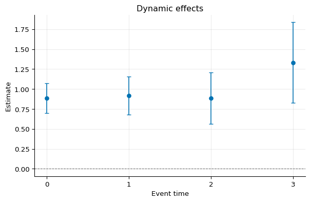
Overall summary of ATT's based on event-study/dynamic aggregation:
  LATT    Std. Error    [95%      Conf. Band]
1.0047        0.1281    0.7537         1.2557  *

Dynamic effects:
  Event time    Estimate    Std. Error    [95% Pointwise    Conf. Band]
           0      0.8868        0.0946            0.7013         1.0723  *
           1      0.9157        0.1215            0.6775         1.1539  *
           2      0.8853        0.1631            0.5656         1.2051  *
           3      1.3310        0.2582            0.8249         1.8371  *
---
Signif. codes: `*' confidence band does not cover 0
Control group: Never treated
Estimation Method: Doubly Robust

fig, ax = dynamic.plot()

Dynamic Balanced Effects

dynamic_bal = idid.agg_latt(res, method="dynamic")
dynamic_bal.summary()

Overall summary of ATT's based on event-study/dynamic aggregation:
  LATT    Std. Error    [95%      Conf. Band]
1.0047        0.1281    0.7537         1.2557  *

Dynamic effects:
  Event time    Estimate    Std. Error    [95% Pointwise    Conf. Band]
           0      0.8868        0.0946            0.7013         1.0723  *
           1      0.9157        0.1215            0.6775         1.1539  *
           2      0.8853        0.1631            0.5656         1.2051  *
           3      1.3310        0.2582            0.8249         1.8371  *
---
Signif. codes: `*' confidence band does not cover 0
Control group: Never treated
Estimation Method: Doubly Robust

fig, ax = dynamic_bal.plot()

Cohort Effects

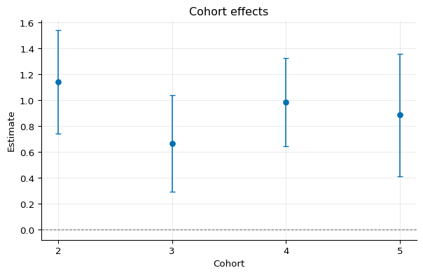
cohort = idid.agg_latt(res, method="cohort")
cohort.summary()

Overall summary of ATT's based on cohort aggregation:
  LATT    Std. Error    [95%      Conf. Band]
0.9182        0.1023    0.7177         1.1187  *

Cohort effects:
  Cohort    Estimate    Std. Error    [95% Pointwise    Conf. Band]
       2      1.1403        0.2037            0.7409         1.5396  *
       3      0.6679        0.1905            0.2945         1.0413  *
       4      0.9850        0.1742            0.6435         1.3265  *
       5      0.8852        0.2399            0.4151         1.3554  *
---
Signif. codes: `*' confidence band does not cover 0
Control group: Never treated
Estimation Method: Doubly Robust

fig, ax = cohort.plot()

Calendar Effects

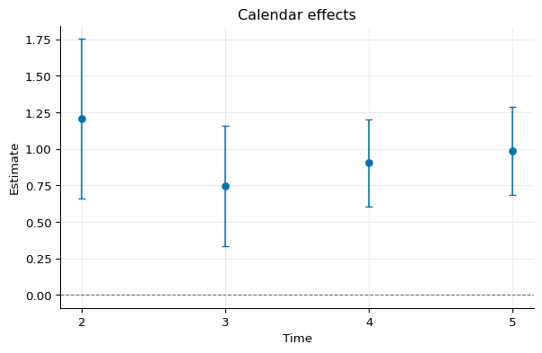
calendar = idid.agg_latt(res, method="calendar")
calendar.summary()

Overall summary of ATT's based on calendar time aggregation:
  LATT    Std. Error    [95%      Conf. Band]
0.9610        0.1189    0.7279         1.1941  *

Time effects:
  Time    Estimate    Std. Error    [95% Pointwise    Conf. Band]
     2      1.2059        0.2793            0.6586         1.7533  *
     3      0.7459        0.2098            0.3346         1.1571  *
     4      0.9057        0.1520            0.6078         1.2036  *
     5      0.9865        0.1540            0.6846         1.2884  *
---
Signif. codes: `*' confidence band does not cover 0
Control group: Never treated
Estimation Method: Doubly Robust

fig, ax = calendar.plot()

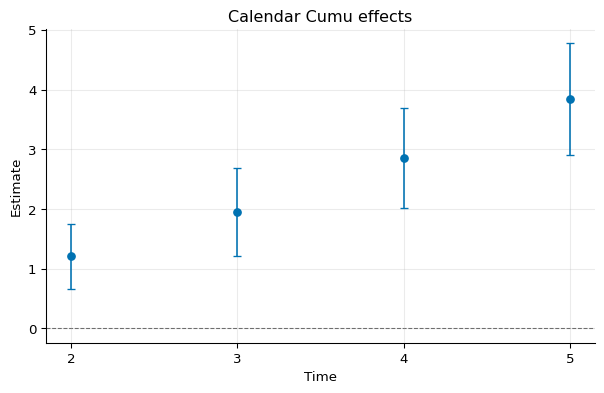
Cumulative Calendar Effects

calendar_cumu = idid.agg_latt(res, method="calendar_cumu")
calendar_cumu.summary()

Overall summary of ATT's based on Calendar_cumu aggregation:
  LATT    Std. Error    [95%      Conf. Band]
2.4648        0.3696    1.7405         3.1891  *

Calendar_cumu effects:
  Calendar_cumu    Estimate    Std. Error    [95% Pointwise    Conf. Band]
              2      1.2059        0.2793            0.6586         1.7533  *
              3      1.9518        0.3764            1.2141         2.6895  *
              4      2.8575        0.4277            2.0193         3.6957  *
              5      3.8440        0.4756            2.9117         4.7762  *
---
Signif. codes: `*' confidence band does not cover 0
Control group: Never treated
Estimation Method: Doubly Robust

fig, ax = calendar_cumu.plot()

Simple Overall Effect

simple = idid.agg_latt(res, method="simple")
simple.summary()

  LATT    Std. Error    [95%      Conf. Band]
0.9386        0.1075    0.7278         1.1494  *

Simultaneous Confidence Bands

Use boot=True to compute multiplier bootstrap standard errors and simultaneous confidence bands.

dynamic_b = idid.agg_latt(
    res,
    method="dynamic",
    boot=True,
    B=999,
)
dynamic_b.summary()

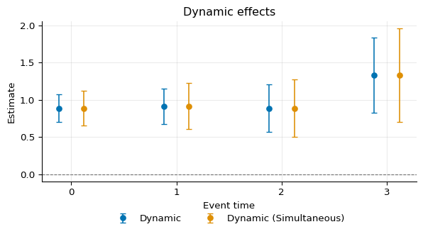
Overall summary of ATT's based on event-study/dynamic aggregation:
  LATT    Std. Error    [95% Simult.    Conf. Band]
1.0047        0.1270          0.7434         1.2660  *

Dynamic effects:
  Event time    Estimate    Std. Error    [95% Simult.    Conf. Band]
           0      0.8868        0.0932          0.6558         1.1178  *
           1      0.9157        0.1240          0.6081         1.2233  *
           2      0.8853        0.1554          0.5000         1.2707  *
           3      1.3310        0.2541          0.7009         1.9611  *
---
Signif. codes: `*' confidence band does not cover 0
Control group: Never treated
Estimation Method: Doubly Robust
Multiplier bootstrap: B=999, c=2.4797, overall c=2.0571

The boot.c value is the critical value used for the simultaneous confidence band.

print(dynamic_b.boot.c)

2.4797294389143825

We can compare the simultaneous confidence bands with the pointwise as:

from idid.plotting import plot_agg
from matplotlib import pyplot as plt

fig, ax = plot_agg(
    [dynamic, dynamic_b],
    labels=[
        "Dynamic",
        "Dynamic (Simultaneous)",
    ],
)