Examples
This page collects a few slightly less standard use cases that build on the main workflow from the quickstart and aggregation pages.
Custom Group Aggregation
You can aggregate cohorts into custom groups by passing a custom_map
to agg_latt(..., method="cohort_custom").
 1import idid
 2
 3df = idid.sim_stag_panel(
 4    n=10_000,
 5    T=5,
 6    E_cohorts=[0, 2, 3, 4, 5],
 7)
 8
 9res = idid.estimate(
10    df,
11    cohort="E",
12    time="t",
13    outcome="Y_t",
14    treatment="D_t",
15    unit="id",
16    covariates=["X"],
17    control="never",
18    method="dr",
19    balanced=True,
20    verbose=False,
21)
22
23custom_map = {
24    2: "2-3",
25    3: "2-3",
26    4: "4-5",
27    5: "4-5",
28}
29
30agg = idid.agg_latt(
31    res,
32    method="cohort_custom",
33    agg_kwargs={"custom_map": custom_map},
34)
35agg.summary()
Overall summary of ATT's based on custom cohort aggregation:
  LATT    Std. Error    [95%      Conf. Band]
1.1750        0.1013    0.9765         1.3734  *

Custom cohort effects:
Cohort      Estimate    Std. Error    [95% Pointwise    Conf. Band]
2-3           0.9925        0.1214            0.7545         1.2304  *
4-5           1.3506        0.1584            1.0402         1.6610  *
---
Signif. codes: `*' confidence band does not cover 0
Control group: Never treated
Estimation Method: Doubly Robust
Compare that to:
1agg = idid.agg_latt(res, method="cohort")
2agg.summary()
Overall summary of ATT's based on cohort aggregation:
  LATT    Std. Error    [95%      Conf. Band]
1.1522        0.0992    0.9577         1.3466  *

Cohort effects:
  Cohort    Estimate    Std. Error    [95% Pointwise    Conf. Band]
       2      0.9999        0.1625            0.6813         1.3185  *
       3      0.9818        0.1793            0.6304         1.3331  *
       4      1.5078        0.2244            1.0680         1.9477  *
       5      1.0982        0.2087            0.6891         1.5072  *
---
Signif. codes: `*' confidence band does not cover 0
Control group: Never treated
Estimation Method: Doubly Robust
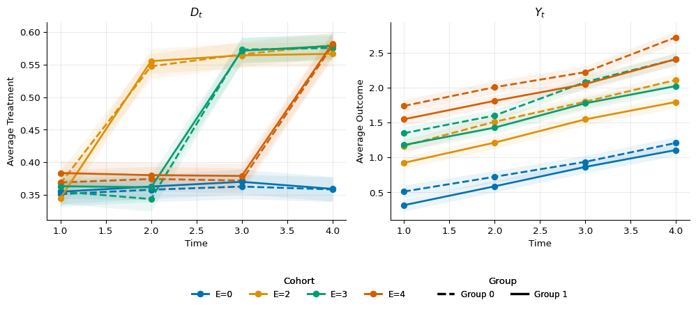
Group Difference Aggregation
To estimate differences between two groups, estimate the cohort-time
LATTs within each group and then call group_diff_idid. The true
difference between the groups equals \(1/2\) for all \((e, t)\).
 1import polars as pl
 2
 3from idid.aggregate import group_diff_idid
 4from idid.plotting import plot_agg, plot_evolution_groups, summarize_evolution
 5
 6df = idid.sim_stag_panel(
 7    n=20_000,
 8    T=4,
 9    E_cohorts=[0, 2, 3, 4],
10    confounded=True,
11    with_group=True,
12)
13print(df.head())
shape: (5, 7)
┌─────┬─────┬─────┬───────────┬─────┬──────────┬─────┐
│ id  ┆ E   ┆ t   ┆ X         ┆ D_t ┆ Y_t      ┆ F   │
│ --- ┆ --- ┆ --- ┆ ---       ┆ --- ┆ ---      ┆ --- │
│ i64 ┆ i64 ┆ i64 ┆ f64       ┆ i64 ┆ f64      ┆ i64 │
╞═════╪═════╪═════╪═══════════╪═════╪══════════╪═════╡
│ 0   ┆ 4   ┆ 1   ┆ 1.285605  ┆ 1   ┆ 7.275993 ┆ 1   │
│ 0   ┆ 4   ┆ 2   ┆ 1.285605  ┆ 0   ┆ 2.930226 ┆ 1   │
│ 0   ┆ 4   ┆ 3   ┆ 1.285605  ┆ 0   ┆ 3.64175  ┆ 1   │
│ 0   ┆ 4   ┆ 4   ┆ 1.285605  ┆ 1   ┆ 7.260314 ┆ 1   │
│ 1   ┆ 4   ┆ 1   ┆ -0.303553 ┆ 1   ┆ 3.297906 ┆ 0   │
└─────┴─────┴─────┴───────────┴─────┴──────────┴─────┘
1gp0 = summarize_evolution(df.filter(pl.col("F").eq(0)))
2gp1 = summarize_evolution(df.filter(pl.col("F").eq(1)))
3fig, ax = plot_evolution_groups(
4    gp0,
5    gp1,
6    include_bands=True,
7)
 1ests = {}
 2for f in [0, 1]:
 3    res = idid.estimate(
 4        df.filter(pl.col("F").eq(f)).with_columns(
 5            id=pl.lit("M" if f == 0 else "F") + pl.col("id").cast(pl.Utf8),
 6        ),
 7        cohort="E",
 8        time="t",
 9        outcome="Y_t",
10        treatment="D_t",
11        unit="id",
12        covariates=["X"],
13        control="never",
14        method="dr",
15        balanced=True,
16        verbose=False,
17    )
18    ests[f] = res
19
20diff = group_diff_idid(ests[1], ests[0])
21
22print(diff.estimates)
23diff.summary()
shape: (6, 7)
┌─────┬─────┬───────────┬──────────┬──────────┬───────────┬───────────┐
│ E   ┆ t   ┆ latt      ┆ denom    ┆ se       ┆ lower     ┆ upper     │
│ --- ┆ --- ┆ ---       ┆ ---      ┆ ---      ┆ ---       ┆ ---       │
│ i64 ┆ i64 ┆ f64       ┆ f64      ┆ f64      ┆ f64       ┆ f64       │
╞═════╪═════╪═══════════╪══════════╪══════════╪═══════════╪═══════════╡
│ 2   ┆ 2   ┆ -0.713377 ┆ 0.188419 ┆ 0.486029 ┆ -1.665993 ┆ 0.239239  │
│ 2   ┆ 3   ┆ -0.721623 ┆ 0.19596  ┆ 0.452582 ┆ -1.608683 ┆ 0.165437  │
│ 2   ┆ 4   ┆ -0.831864 ┆ 0.211267 ┆ 0.415799 ┆ -1.64683  ┆ -0.016897 │
│ 3   ┆ 3   ┆ -0.747214 ┆ 0.214008 ┆ 0.41707  ┆ -1.564672 ┆ 0.070243  │
│ 3   ┆ 4   ┆ -0.991648 ┆ 0.225592 ┆ 0.391804 ┆ -1.759584 ┆ -0.223713 │
│ 4   ┆ 4   ┆ -0.591208 ┆ 0.211862 ┆ 0.417223 ┆ -1.408965 ┆ 0.226549  │
└─────┴─────┴───────────┴──────────┴──────────┴───────────┴───────────┘
Cohort-Time Local Average Treatment Effects on the Treated:
 E   t    AET(e, t)   LATT(e, t)   Std. Error   [95% Pointwise.   Conf. Band]
 2   2       0.1884      -0.7134       0.4860           -1.6660        0.2392
 2   3       0.1960      -0.7216       0.4526           -1.6087        0.1654
 2   4       0.2113      -0.8319       0.4158           -1.6468       -0.0169  *
 3   3       0.2140      -0.7472       0.4171           -1.5647        0.0702
 3   4       0.2256      -0.9916       0.3918           -1.7596       -0.2237  *
 4   4       0.2119      -0.5912       0.4172           -1.4090        0.2265
---
Signif. codes: `*' confidence band does not cover 0
Control group: Never treated
Estimation Method: Doubly Robust
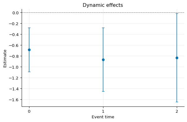
Aggregated dynamic effects:
1agg = idid.agg_latt(diff, method="dynamic")
2agg.summary()
Overall summary of ATT's based on event-study/dynamic aggregation:
   LATT    Std. Error    [95%      Conf. Band]
-0.7932        0.2551   -1.2933        -0.2932  *

Dynamic effects:
  Event time    Estimate    Std. Error    [95% Pointwise    Conf. Band]
           0     -0.6834        0.2080           -1.0910        -0.2758  *
           1     -0.8644        0.2980           -1.4485        -0.2802  *
           2     -0.8319        0.4158           -1.6468        -0.0169  *
---
Signif. codes: `*' confidence band does not cover 0
Control group: Never treated
Estimation Method: Doubly Robust
1fig, ax = plot_agg([agg])
1agg_diff = idid.agg_latt(diff, method="dynamic", boot=True)
2agg_diff.summary()
Overall summary of ATT's based on event-study/dynamic aggregation:
   LATT    Std. Error    [95% Simult.    Conf. Band]
-0.7932        0.2619         -1.3063        -0.2802  *

Dynamic effects:
  Event time    Estimate    Std. Error    [95% Simult.    Conf. Band]
           0     -0.6834        0.2119         -1.1694        -0.1975  *
           1     -0.8644        0.3044         -1.5624        -0.1663  *
           2     -0.8319        0.4086         -1.7690         0.1053
---
Signif. codes: `*' confidence band does not cover 0
Control group: Never treated
Estimation Method: Doubly Robust
Multiplier bootstrap: B=1000, c=2.2934, overall c=1.9588
Compare that to:
1agg0 = idid.agg_latt(ests[0], method="dynamic", boot=True)
2agg0.summary()
Overall summary of ATT's based on event-study/dynamic aggregation:
  LATT    Std. Error    [95% Simult.    Conf. Band]
1.1506        0.1841          0.7958         1.5054  *

Dynamic effects:
  Event time    Estimate    Std. Error    [95% Simult.    Conf. Band]
           0      1.0224        0.1550          0.6773         1.3675  *
           1      1.2295        0.2259          0.7265         1.7325  *
           2      1.2000        0.2980          0.5366         1.8633  *
---
Signif. codes: `*' confidence band does not cover 0
Control group: Never treated
Estimation Method: Doubly Robust
Multiplier bootstrap: B=1000, c=2.2264, overall c=1.9274
1agg1 = idid.agg_latt(ests[1], method="dynamic", boot=True)
2agg1.summary()
Overall summary of ATT's based on event-study/dynamic aggregation:
  LATT    Std. Error    [95% Simult.    Conf. Band]
0.3494        0.1739         -0.0236         0.7224

Dynamic effects:
  Event time    Estimate    Std. Error    [95% Simult.    Conf. Band]
           0      0.3214        0.1408          0.0042         0.6387  *
           1      0.3587        0.2134         -0.1220         0.8394
           2      0.3681        0.2922         -0.2901         1.0263
---
Signif. codes: `*' confidence band does not cover 0
Control group: Never treated
Estimation Method: Doubly Robust
Multiplier bootstrap: B=1000, c=2.2528, overall c=2.1445
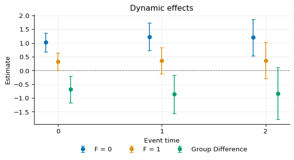
We can plot the three aggregated objects:
1fig, ax = plot_agg(
2    [agg0, agg1, agg_diff],
3    labels=[
4        "F = 0",
5        "F = 1",
6        "Group Difference",
7    ],
8)
Introspection of estimates
The implementation allows for inspection of specific \(LATT(e, t)\)
estimates. After calling idid.estimate, the cell-level results are
stored in the latts dictionary of the returned object. This is useful
when you want to inspect one particular effect and see which treated and
control observations entered that comparison.
 1from idid._types import FailedLATT
 2from idid.estimators import get_controls
 3
 4res = idid.estimate(
 5    idid.sim_stag_panel(
 6        n=10_000,
 7        T=5,
 8        E_cohorts=[2, 3, 4, 5],
 9    ),
10    cohort="E",
11    time="t",
12    outcome="Y_t",
13    treatment="D_t",
14    unit="id",
15    covariates=["X"],
16    control="notyet",
17    method="dr",
18    balanced=True,
19    verbose=False,
20)
21
22e = 2
23t = 3
24latt = res.latts[(e, t)]
25if isinstance(latt, FailedLATT):
26    raise ValueError("Failed LATT estimation")
27
28print(latt)
LATT(g=2, t=3, latt=float64(), num=float64(), denom=float64(), ns=7417, ids=DataFrame[7417x2; id, E], IF=ndarray(7417, 1), IF_aet=ndarray(7417, 1), extra=dict[num, den])
Each LATT object stores the underlying unit-period ids used for that
comparison. In the ids data frame, E = 1 denotes treated
observations and E = 0 denotes controls.
1print(latt.ids.head())
2print(latt.ids["E"].value_counts())
shape: (5, 2)
┌─────┬─────┐
│ id  ┆ E   │
│ --- ┆ --- │
│ i64 ┆ i8  │
╞═════╪═════╡
│ 1   ┆ 1   │
│ 2   ┆ 0   │
│ 3   ┆ 0   │
│ 4   ┆ 0   │
│ 5   ┆ 0   │
└─────┴─────┘
shape: (2, 2)
┌─────┬───────┐
│ E   ┆ count │
│ --- ┆ ---   │
│ i8  ┆ u32   │
╞═════╪═══════╡
│ 0   ┆ 4945  │
│ 1   ┆ 2472  │
└─────┴───────┘
A small helper returns the control units for a given LATT object and
IDidResult.
1controls = get_controls(latt, res).sort("id")
2print(controls.head())
shape: (5, 2)
┌─────┬─────┐
│ id  ┆ E   │
│ --- ┆ --- │
│ i64 ┆ i64 │
╞═════╪═════╡
│ 2   ┆ 5   │
│ 3   ┆ 4   │
│ 4   ┆ 5   │
│ 5   ┆ 4   │
│ 6   ┆ 5   │
└─────┴─────┘
1print(f"#Controls = {controls.shape[0]}")
2print(controls[res.dp.e_col].value_counts().sort(res.dp.e_col))
#Controls = 4945
shape: (2, 2)
┌─────┬───────┐
│ E   ┆ count │
│ --- ┆ ---   │
│ i64 ┆ u32   │
╞═════╪═══════╡
│ 4   ┆ 2453  │
│ 5   ┆ 2492  │
└─────┴───────┘
I.e. the not-yet-exposed controls for \(\hat{LATT}(2, 3)\) are evenly distributed across the cohorts \(E \in \{4, 5\}\).