tabx - compose LaTeX tables using booktabs in Python

tabular + booktabs is all you need
tabxis a Python library for creating LaTeX tables using the booktabs packageFeatures include:
concatenate
Tables (and other table-related LaTeX objects) horizontally and vertically using overloaded|and/operatorsslice tables using numpy-like indexing e.g.
table[1:, 2:]no external dependencies
For a quick overview of functionality, see showcase
For a more in-depth tutorial, see tutorial
For some wisdom, see wisdom from bookstabs
For a list of examples, see examples
See also the documentation
Installation
uv pip install tabx-py
Showcase
1from tabx import Cell, Table, Cmidrule, Midrule, multirow_column, multicolumn_row
2
3C = Cell
4
5base = Table.from_cells(
6 [
7 [C(3.14), C(3.14), C(3.14), C(3.14)],
8 [C(1.62), C(1.62), C(1.62), C(1.62)],
9 [C(1.41), C(1.41), C(1.41), C(1.41)],
10 [C(2.72), C(2.72), C(2.72), C(2.72)],
11 ]
12)
13row_labels = Table.from_cells(
14 [
15 C(r"$\sigma = 0.1$"),
16 C(r"$\sigma = 0.3$"),
17 C(r"$\eta = 0.1$"),
18 C(r"$\eta = 0.3$"),
19 ],
20)
21header = multicolumn_row(r"$\beta$", 2, pad_before=2) | multicolumn_row(r"$\gamma$", 2)
22mr = multirow_column(r"$R_{1}$", 4)
23cmrs = Cmidrule(3, 4, "lr") | Cmidrule(5, 6, "lr")
24# Stack header on top of Cmidrules; stack row labels onto table from the left
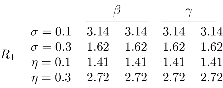
25tab = header / cmrs / (mr | row_labels | base)
26tab.print() # Print table to stdout
\begin{tabular}{@{}cccccc@{}}
  \toprule
   &  & \multicolumn{2}{c}{$\beta$} & \multicolumn{2}{c}{$\gamma$} \\
  \cmidrule(lr){3-4}
  \cmidrule(lr){5-6}
  \multirow{4}{*}{$R_{1}$} & $\sigma = 0.1$ & 3.14 & 3.14 & 3.14 & 3.14 \\
   & $\sigma = 0.3$ & 1.62 & 1.62 & 1.62 & 1.62 \\
   & $\eta = 0.1$ & 1.41 & 1.41 & 1.41 & 1.41 \\
   & $\eta = 0.3$ & 2.72 & 2.72 & 2.72 & 2.72 \\
  \bottomrule
\end{tabular}
Compiling the table and converting to PNG yields:
1# Add some more complexity to the previous table
2row_labels2 = Table.from_cells(
3 [
4 C(r"$\xi = 0.1$"),
5 C(r"$\xi = 0.3$"),
6 C(r"$\delta = 0.1$"),
7 C(r"$\delta = 0.3$"),
8 ],
9)
10header2 = multicolumn_row(r"$\theta$", 2) | multicolumn_row(r"$\mu$", 2)
11mr = multirow_column(r"$R_{2}$", 4)
12tab2 = mr | row_labels2 | base
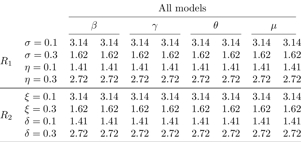
13concat_tab = (
14 # Stack header with Cmidrule above all columns
15 (multicolumn_row("All models", 8, pad_before=2) / Cmidrule(3, 10))
16 / (
17 # Stack tables vertically with Midrule in between
18 (tab / Midrule() / tab2)
19 # Stack the resulting table horizontally with the one below
20 | (
21 # Slice tables and stack new header on top
22 # Cmidrules start from 1 while no row labels for the right table
23 header2
24 / (Cmidrule(1, 2, "lr") | Cmidrule(3, 4, "lr"))
25 / tab[2:, 2:] # Previous table sliced
26 / Midrule()
27 / tab2[:, 2:] # New table sliced
28 )
29 )
30).set_align(2 * "l" + 8 * "c")
31concat_tab.print()
\begin{tabular}{@{}llcccccccc@{}}
  \toprule
   &  & \multicolumn{8}{c}{All models} \\
  \cmidrule(lr){3-10}
   &  & \multicolumn{2}{c}{$\beta$} & \multicolumn{2}{c}{$\gamma$} & \multicolumn{2}{c}{$\theta$} & \multicolumn{2}{c}{$\mu$} \\
  \cmidrule(lr){3-4}
  \cmidrule(lr){5-6}
  \cmidrule(lr){7-8}
  \cmidrule(lr){9-10}
  \multirow{4}{*}{$R_{1}$} & $\sigma = 0.1$ & 3.14 & 3.14 & 3.14 & 3.14 & 3.14 & 3.14 & 3.14 & 3.14 \\
   & $\sigma = 0.3$ & 1.62 & 1.62 & 1.62 & 1.62 & 1.62 & 1.62 & 1.62 & 1.62 \\
   & $\eta = 0.1$ & 1.41 & 1.41 & 1.41 & 1.41 & 1.41 & 1.41 & 1.41 & 1.41 \\
   & $\eta = 0.3$ & 2.72 & 2.72 & 2.72 & 2.72 & 2.72 & 2.72 & 2.72 & 2.72 \\
  \midrule
  \multirow{4}{*}{$R_{2}$} & $\xi = 0.1$ & 3.14 & 3.14 & 3.14 & 3.14 & 3.14 & 3.14 & 3.14 & 3.14 \\
   & $\xi = 0.3$ & 1.62 & 1.62 & 1.62 & 1.62 & 1.62 & 1.62 & 1.62 & 1.62 \\
   & $\delta = 0.1$ & 1.41 & 1.41 & 1.41 & 1.41 & 1.41 & 1.41 & 1.41 & 1.41 \\
   & $\delta = 0.3$ & 2.72 & 2.72 & 2.72 & 2.72 & 2.72 & 2.72 & 2.72 & 2.72 \\
  \bottomrule
\end{tabular}
Compiling the table and converting to PNG yields:
Tutorial
Cell, Table, and concatenation
1from tabx import Cell
2from tabx import utils
The most basic object is a Cell
1cell = Cell("1")
2cell
Cell(value="1", multirow=1, multicolumn=1)
Rendering a cell returns it values as a str
1cell.render()
'1'
1cell = Cell(r"$\alpha$")
2cell.render()
'$\\alpha$'
Cells can be concatenated with other cells. Concatenating three cells
horizontally with the | operator yields a Table object of dimension
(1, 3)
1tab = Cell("1") | Cell("2") | Cell("3")
2tab
Table(nrows=1, ncols=3)
Rendering this yields a str with the three cells concatenated wrapped
inside a tabular environment ready to be used in a LaTeX document.
1tab.render()
'\\begin{tabular}{@{}ccc@{}}\n \\toprule\n 1 & 2 & 3 \\\\\n \\bottomrule\n\\end{tabular}'
Can also be done vertically with the / operator yielding a Table
object of dimension (3, 1)
1tab_other = Cell("1") / Cell("2") / Cell("3")
2tab_other
Table(nrows=3, ncols=1)
We can concatenate a Table horizontally to stack the tables above each
other. This is done using the / operator.
1stacked_tab = tab / tab
2stacked_tab
Table(nrows=2, ncols=3)
And we can concatenate another table onto it from below and then the other from the right
1stacked_tab2 = (stacked_tab / tab) | tab_other
2stacked_tab2
Table(nrows=3, ncols=4)
To print out how the table looks like, we can use the print method;
this does not return anything but prints out the object to the console.
1stacked_tab2.print()
\begin{tabular}{@{}cccc@{}}
  \toprule
  1 & 2 & 3 & 1 \\
  1 & 2 & 3 & 2 \\
  1 & 2 & 3 & 3 \\
  \bottomrule
\end{tabular}
Say we want some columns name onto this table. This can be done:
1stacked_tab3 = (Cell("A") | Cell("B") | Cell("C") | Cell("D")) / stacked_tab2
2stacked_tab3.print()
\begin{tabular}{@{}cccc@{}}
  \toprule
  A & B & C & D \\
  1 & 2 & 3 & 1 \\
  1 & 2 & 3 & 2 \\
  1 & 2 & 3 & 3 \\
  \bottomrule
\end{tabular}
Maybe we want a Midrule underneath the column names. This can be done
as:
1from tabx import Midrule
2
3stacked_tab3 = (
4    (Cell("A") | Cell("B") | Cell("C") | Cell("D")) / Midrule() / stacked_tab2
5)
6stacked_tab3.print()
\begin{tabular}{@{}cccc@{}}
  \toprule
  A & B & C & D \\
  \midrule
  1 & 2 & 3 & 1 \\
  1 & 2 & 3 & 2 \\
  1 & 2 & 3 & 3 \\
  \bottomrule
\end{tabular}
Let add some variable names on the left side. We can construct a column as:
1row_labels = (
2    # The header row and Midrule row shouldn't get a label hence empty cells
3    Cell("") / Cell("") / Cell("Var1") / Cell("Var2") / Cell("Var3")
4)
5stacked_tab3 = row_labels | stacked_tab3
6stacked_tab3.print()
\begin{tabular}{@{}ccccc@{}}
  \toprule
   & A & B & C & D \\
  \midrule
  Var1 & 1 & 2 & 3 & 1 \\
  Var2 & 1 & 2 & 3 & 2 \\
  Var3 & 1 & 2 & 3 & 3 \\
  \bottomrule
\end{tabular}
If you have a LaTeX compiler in your path, you can compile the table to
a PDF and convert it to a PNG using tabx.utils.compile_table and
tabx.utils.pdf_to_png respectively.
1file = utils.compile_table(
2    stacked_tab2.render(),
3    silent=True,
4    name="tutorial",
5    output_dir=utils.proj_folder().joinpath("figs"),
6)
7_ = utils.pdf_to_png(file)
Compiling the table to PDF and converting it to PNG yields:

Slicing tables
Tables can be sliced like numpy arrays.
1# Slice out the row label column
2sliced_tab = stacked_tab3[:, 1:]
3sliced_tab
Table(nrows=5, ncols=4)
1sliced_tab.print()
\begin{tabular}{@{}cccc@{}}
  \toprule
  A & B & C & D \\
  \midrule
  1 & 2 & 3 & 1 \\
  1 & 2 & 3 & 2 \\
  1 & 2 & 3 & 3 \\
  \bottomrule
\end{tabular}
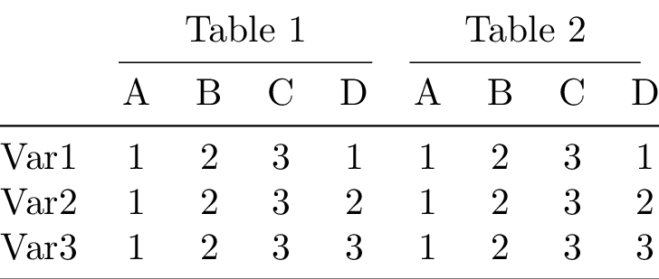
Lets concatenate the sliced table to the original table, add a header
above the columns of each concatenated table and two Cmidrules between
to distinguish the two tables.
 1from tabx import Cmidrule
 2
 3tab = (
 4    # Add a header row; one empty cell for the row label column
 5    (Cell("") | Cell("Table 1", multicolumn=4) | Cell("Table 2", multicolumn=4))
 6    # Insert Cmidrules after columns
 7    / (Cmidrule(2, 5, trim="lr") | Cmidrule(6, 9, trim="lr"))
 8    # Stack header row and Cmidrules above the concatenated tables
 9    / (stacked_tab3 | sliced_tab)
10    # Left align the first column and center the rest
11    .set_align("l" + "c" * 8)
12)
13tab.print()
14file = utils.compile_table(
15    tab.render(),
16    silent=True,
17    name="tutorial2",
18    output_dir=utils.proj_folder().joinpath("figs"),
19)
20_ = utils.pdf_to_png(file)
\begin{tabular}{@{}ccccccccc@{}}
  \toprule
   & \multicolumn{4}{c}{Table 1} & \multicolumn{4}{c}{Table 2} \\
  \cmidrule(lr){2-5}
  \cmidrule(lr){6-9}
   & A & B & C & D & A & B & C & D \\
  \midrule
  Var1 & 1 & 2 & 3 & 1 & 1 & 2 & 3 & 1 \\
  Var2 & 1 & 2 & 3 & 2 & 1 & 2 & 3 & 2 \\
  Var3 & 1 & 2 & 3 & 3 & 1 & 2 & 3 & 3 \\
  \bottomrule
\end{tabular}
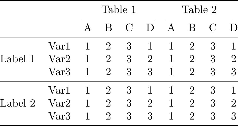
Okay let’s have some fun. We’ll slice out the upper part of the previous table, concatenate the sliced table onto it from below and then concatenate a column of multirow labels on the left. Let’s see it in action instead of the just read word salad:
 1from tabx import empty_table
 2
 3multirow_labels = (
 4    empty_table(3, 1)
 5    / Midrule()
 6    # A multirow label spanning 3 rows should be followed by 2 empty cells
 7    / (Cell("Label 1", multirow=3) / empty_table(2, 1))
 8    / Midrule()
 9    / (Cell("Label 2", multirow=3) / empty_table(2, 1))
10)
11tab_new = multirow_labels | (tab / tab[3:, :])
12tab_new.print()
13file = utils.compile_table(
14    tab_new.render(),
15    silent=True,
16    name="tutorial3",
17    output_dir=utils.proj_folder().joinpath("figs"),
18)
19_ = utils.pdf_to_png(file)
\begin{tabular}{@{}cccccccccc@{}}
  \toprule
   &  & \multicolumn{4}{c}{Table 1} & \multicolumn{4}{c}{Table 2} \\
  \cmidrule(lr){3-6}
  \cmidrule(lr){7-10}
   &  & A & B & C & D & A & B & C & D \\
  \midrule
  \multirow{3}{*}{Label 1} & Var1 & 1 & 2 & 3 & 1 & 1 & 2 & 3 & 1 \\
   & Var2 & 1 & 2 & 3 & 2 & 1 & 2 & 3 & 2 \\
   & Var3 & 1 & 2 & 3 & 3 & 1 & 2 & 3 & 3 \\
  \midrule
  \multirow{3}{*}{Label 2} & Var1 & 1 & 2 & 3 & 1 & 1 & 2 & 3 & 1 \\
   & Var2 & 1 & 2 & 3 & 2 & 1 & 2 & 3 & 2 \\
   & Var3 & 1 & 2 & 3 & 3 & 1 & 2 & 3 & 3 \\
  \bottomrule
\end{tabular}
1from tabx import Table
2
3# Renders the table body without the tabular environment
4print(tab_new.render_body())
 &  & \multicolumn{4}{c}{Table 1} & \multicolumn{4}{c}{Table 2} \\
\cmidrule(lr){3-6}
\cmidrule(lr){7-10}
 &  & A & B & C & D & A & B & C & D \\
\midrule
\multirow{3}{*}{Label 1} & Var1 & 1 & 2 & 3 & 1 & 1 & 2 & 3 & 1 \\
 & Var2 & 1 & 2 & 3 & 2 & 1 & 2 & 3 & 2 \\
 & Var3 & 1 & 2 & 3 & 3 & 1 & 2 & 3 & 3 \\
\midrule
\multirow{3}{*}{Label 2} & Var1 & 1 & 2 & 3 & 1 & 1 & 2 & 3 & 1 \\
 & Var2 & 1 & 2 & 3 & 2 & 1 & 2 & 3 & 2 \\
 & Var3 & 1 & 2 & 3 & 3 & 1 & 2 & 3 & 3 \\
Custom render function
A custom rendering function can be used to render the body of a table.
 1def render_body_simple(table: Table):
 2    if not (align := table.align):
 3        align = "c" * table.ncols
 4    return "\n".join(
 5        [
 6            r"\begin{tabular}{" + align + r"}",
 7            table.render_body(),
 8            r"\end{tabular}",
 9        ]
10    )
11
12
13print(tab_new.render(custom_render=render_body_simple))
\begin{tabular}{cccccccccc}
 &  & \multicolumn{4}{c}{Table 1} & \multicolumn{4}{c}{Table 2} \\
\cmidrule(lr){3-6}
\cmidrule(lr){7-10}
 &  & A & B & C & D & A & B & C & D \\
\midrule
\multirow{3}{*}{Label 1} & Var1 & 1 & 2 & 3 & 1 & 1 & 2 & 3 & 1 \\
 & Var2 & 1 & 2 & 3 & 2 & 1 & 2 & 3 & 2 \\
 & Var3 & 1 & 2 & 3 & 3 & 1 & 2 & 3 & 3 \\
\midrule
\multirow{3}{*}{Label 2} & Var1 & 1 & 2 & 3 & 1 & 1 & 2 & 3 & 1 \\
 & Var2 & 1 & 2 & 3 & 2 & 1 & 2 & 3 & 2 \\
 & Var3 & 1 & 2 & 3 & 3 & 1 & 2 & 3 & 3 \\
\end{tabular}
Utility functions
The function empty_table is convienient for creating empty cells of
dimension (nrows, ncols) as fillers.
1n, m = 3, 5
2empty_table(n, m)
Table(nrows=3, ncols=5)
The notation for the multirow cells above is a bit verbose. The function
multirow_column is a wrapper for creating a multirow column with
padding before and after the multirow cell.
1from tabx import multirow_column
2
3mr = multirow_column("Label1", multirow=3, pad_before=2, pad_after=2)
4print(mr)
Columns(nrows=7, ncols=1)
1mr.print()
 \\
 \\
\multirow{3}{*}{Label1} \\
 \\
 \\
 \\
 \\
We can write the multirow_labels column from before as:
 1multirow_labels_succ = (
 2    # A multirow label spanning 3 rows should be followed by 2 empty cells
 3    empty_table(3, 1)
 4    / Midrule()
 5    / multirow_column("Label 1", multirow=3)
 6    / Midrule()
 7    / multirow_column("Label 2", multirow=3)
 8)
 9
10print(multirow_labels_succ.rows == multirow_labels.rows)
True
Wisdom from bookstabs
You will not go far wrong if you remember two simple guidelines at all times:
Never, ever use vertical rules.
Never use double rules.
See Section 2 here for more wisdom.
Examples
Simple table
 1import tabx
 2from tabx import ColMap, RowMap
 3
 4tab = tabx.simple_table(
 5    values=[
 6        [3.14, 3.14, 3.14, 3.14],
 7        [1.62, 1.62, 1.62, 1.62],
 8        [1.41, 1.41, 1.41, 1.41],
 9        [2.72, 2.72, 2.72, 2.72],
10    ],
11    col_maps=[ColMap({(1, 2): r"$\beta$", (3, 4): r"$\gamma$"})],
12    row_maps=[
13        RowMap({(1, 4): r"$R_{1}$"}),
14        RowMap(
15            {
16                (1, 1): r"$\sigma = 0.1$",
17                (2, 2): r"$\sigma = 0.3$",
18                (3, 3): r"$\eta = 0.1$",
19                (4, 4): r"$\eta = 0.3$",
20            }
21        ),
22    ],
23)
Compiling the table and converting to PNG yields:

equivalent to the image from the Showcase.
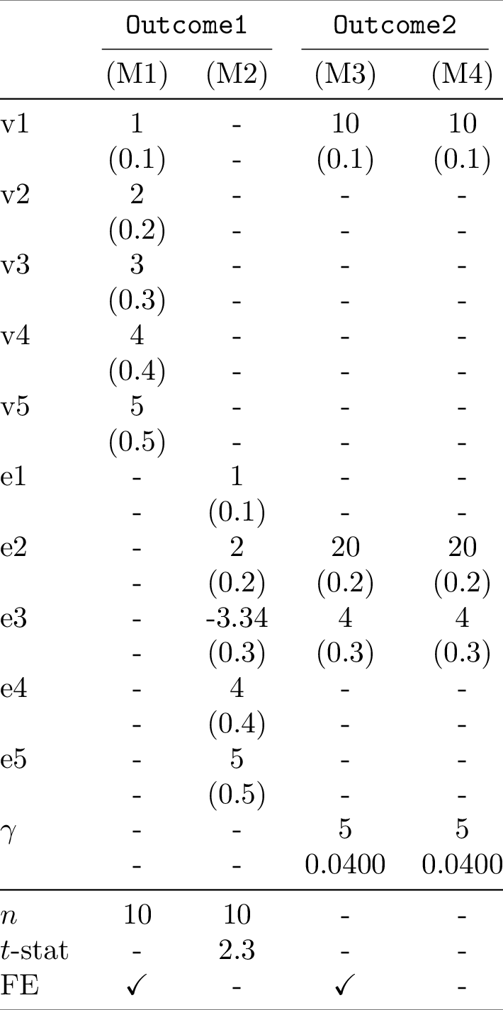
Models estimates and standard errors
Model results dictionary passing
 1import tabx
 2from tabx import ColMap, utils
 3
 4
 5m1 = {
 6    "variable": ["v1", "v2", "v3", "v4", "v5"],
 7    "estimates": [1, 2, 3, 4, 5],
 8    "se": [0.1, 0.2, 0.3, 0.4, 0.5],
 9    "extra_data": {
10        r"$n$": 10,
11        "FE": r"\checkmark",
12    },
13}
14m2 = {
15    "variable": ["e1", "e2", "e3", "e4", "e5"],
16    "estimates": [1, 2, -3.34, 4, 5],
17    "se": [0.1, 0.2, 0.3, 0.4, 0.5],
18    "extra_data": {
19        r"$n$": 10,
20        "$t$-stat": 2.3,
21        "FE": "-",
22    },
23}
24m3 = {
25    "variable": ["v1", "e2", "e3", r"$\gamma$"],
26    "estimates": [10, 20, 4, 5],
27    "se": [0.1, 0.2, 0.3, "0.0400"],
28    "extra_data": {
29        "FE": r"\checkmark",
30    },
31}
32m4 = {
33    "variable": ["v1", "e2", "e3", r"$\gamma$"],
34    "estimates": [10, 20, 4, 5],
35    "se": [0.1, 0.2, 0.3, "0.0400"],
36}
37mod1 = tabx.ModelData.from_dict(m1, name="(M1)")
38mod2 = tabx.ModelData.from_dict(m2, name="(M2)")
39mod3 = tabx.ModelData.from_dict(m3, name="(M3)")
40mod4 = tabx.ModelData.from_dict(m4, name="(M4)")
41models = [mod1, mod2, mod3, mod4]
42
43variables = (
44    ["v1", "v2", "v3", "v4", "v5"] + ["e1", "e2", "e3", "e4", "e5"] + [r"$\gamma$"]
45)
46order_map = dict(zip(variables, range(len(variables)))) | {
47    "session": 0,
48    r"$n$": 1,
49    "$t$-stat": 2,
50}
51tab = tabx.models_table(
52    models,
53    col_maps=ColMap(
54        mapping={
55            (1, 2): r"\texttt{Outcome1}",
56            (3, 4): r"\texttt{Outcome2}",
57        }
58    ),
59    var_name="",
60    order_map=order_map,
61    fill_value="-",
62)
Model results from values
Create model table quickly from a polars.DataFrame using tabx. We
assume the columns are stacked as pairs of estimates and standard errors
for each model.
 1import polars as pl
 2import tabx
 3from tabx import ModelData, utils
 4
 5data = pl.DataFrame(
 6    [
 7        ["$x_1$", -0.44, 1.14, 1.04, 1.12, 0.56, 0.98, -0.25, -0.21],
 8        ["$x_2$", 0.58, -0.63, -0.92, 0.74, 0.45, -0.67, 0.33, 0.12],
 9        ["$x_3$", 0.64, -1.0, 1.15, 0.78, 0.34, -0.89, 0.22, 0.44],
10        ["$x_4$", -0.43, 1.02, 1.76, -0.68, 0.22, 0.45, 0.11, -0.33],
11        ["$x_5$", 0.1, 0.63, -0.35, -0.21, 0.15, 0.33, -0.12, 0.44],
12        ["$x_6$", 0.06, 0.98, 0.56, -0.25, 0.12, 0.44, 0.22, -0.11],
13        ["$x_7$", -1.49, -1.8, 0.8, -0.23, 0.67, 0.55, 0.33, -0.44],
14        ["$x_8$", -1.91, -1.42, -0.3, 0.25, 0.33, 0.22, 0.11, -0.55],
15    ],
16    schema=[
17        "variable",
18        "ests1",
19        "ses1",
20        "ests2",
21        "ses2",
22        "ests3",
23        "ses3",
24        "ests4",
25        "ses4",
26    ],
27    orient="row",
28)
29
30desc_datas = ModelData.from_values(
31    data.rows(),
32    model_names=["M1", "M2", "M3", "M4"],  # Exclude 'variable' column
33    extras=[
34        {"n": 10, "misc": 1},
35        {"n": 20, "misc": 0},
36        {"n": 50, "optimizer": "sgd"},
37        {"n": 25, "optimizer": "sgd"},
38    ],
39)
40tab = tabx.models_table(
41    desc_datas,
42    col_maps=tabx.ColMap(mapping={(1, 2): "OLS", (3, 4): "Logistic"}),
43    include_midrule=True,
44    fill_value="-",
45    var_name="",
46    order_map={"n": 0, "misc": 1, "optimizer": 2},
47)
Compiling the table to PDF and converting it to PNG yields:
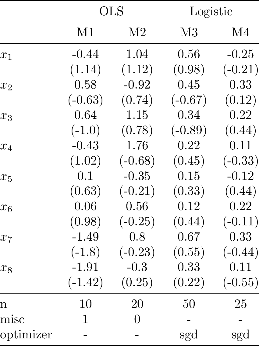
The downside of this approach is that the estimates and standard errors in each row are for the same variable. For the case with many models and many variables the dictionary passing approach is more flexible.
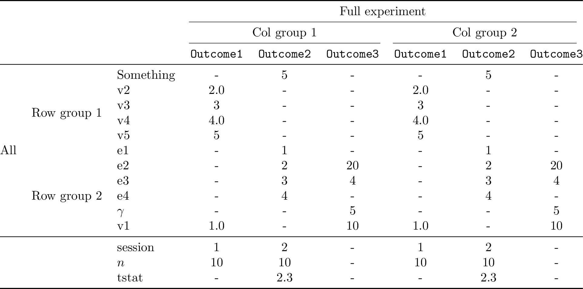
Descriptive statistics
Descriptive statistics dictionary passing
 1import tabx
 2from tabx import ColMap, RowMap, utils
 3
 4
 5m1 = {
 6    "variable": ["v1", "v2", "v3", "v4", "v5"],
 7    "values": [1.0, 2.0, 3, 4.0, 5],
 8    "extra_data": {
 9        r"$n$": 10,
10        "session": 1,
11    },
12}
13m2 = {
14    "variable": ["e1", "e2", "e3", "e4", "Something"],
15    "values": [1, 2, 3, 4, 5],
16    "extra_data": {
17        r"$n$": 10,
18        "tstat": 2.3,
19        "session": 2,
20    },
21}
22m3 = {
23    "variable": ["v1", "e2", "e3", r"$\gamma$"],
24    "values": [10, 20, 4, 5],
25    "se": [0.1, 0.2, 0.3, "0.0400"],
26}
27
28mod1 = tabx.DescData.from_dict(m1, name=r"\texttt{Outcome1}")
29mod2 = tabx.DescData.from_dict(m2, name=r"\texttt{Outcome2}")
30mod3 = tabx.DescData.from_dict(m3, name=r"\texttt{Outcome3}")
31descs = [mod1, mod2, mod3, mod1, mod2, mod3]
32
33variables = (
34    ["Something", "v2", "v3", "v4", "v5"]
35    + ["e1", "e2", "e3", "e4", "e5"]
36    + [r"$\gamma$"]
37)
38order_map = dict(zip(variables, range(len(variables)))) | {
39    "session": 0,
40    r"$n$": 1,
41    "tstat": 2,
42}
43
44
45tab = tabx.descriptives_table(
46    descs,
47    col_maps=[
48        ColMap(
49            mapping={
50                (1, 6): r"Full experiment",
51            },
52            include_cmidrule=True,
53        ),
54        ColMap(
55            mapping={
56                (1, 3): r"Col group 1",
57                (4, 6): r"Col group 2",
58            },
59            include_cmidrule=True,
60        ),
61    ],
62    order_map=order_map,
63    include_header=True,
64    include_extra=True,
65    row_maps=[
66        RowMap(
67            {
68                (1, 11): r"All",
69            }
70        ),
71        RowMap(
72            {
73                (1, 6): r"Row group 1",
74                (7, 11): r"Row group 2",
75            }
76        ),
77    ],
78    fill_value="-",
79)
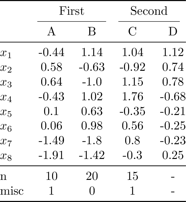
Descriptive statistics from values
Create descriptive table quickly from a polars.DataFrame using tabx.
 1import polars as pl
 2import tabx
 3from tabx import DescData, utils
 4
 5data = pl.DataFrame(
 6    [
 7        ["$x_1$", -0.44, 1.14, 1.04, 1.12],
 8        ["$x_2$", 0.58, -0.63, -0.92, 0.74],
 9        ["$x_3$", 0.64, -1.0, 1.15, 0.78],
10        ["$x_4$", -0.43, 1.02, 1.76, -0.68],
11        ["$x_5$", 0.1, 0.63, -0.35, -0.21],
12        ["$x_6$", 0.06, 0.98, 0.56, -0.25],
13        ["$x_7$", -1.49, -1.8, 0.8, -0.23],
14        ["$x_8$", -1.91, -1.42, -0.3, 0.25],
15    ],
16    schema=["variable", "A", "B", "C", "D"],
17    orient="row",
18)
19
20desc_datas = DescData.from_values(
21    data.rows(),
22    column_names=data.columns[1:],  # Exclude 'variable' column
23    extras=[
24        {"n": 10, "misc": 1},
25        {"n": 20, "misc": 0},
26        {"n": 15, "misc": 1},
27    ],
28)
29tab = tabx.descriptives_table(
30    desc_datas,
31    col_maps=tabx.ColMap(
32        mapping={
33            (1, 2): "First",
34            (3, 4): "Second",
35        }
36    ),
37    include_midrule=True,
38    fill_value="-",
39    order_map={"n": 0, "misc": 1},
40)
Compiling the table to PDF and converting it to PNG yields:
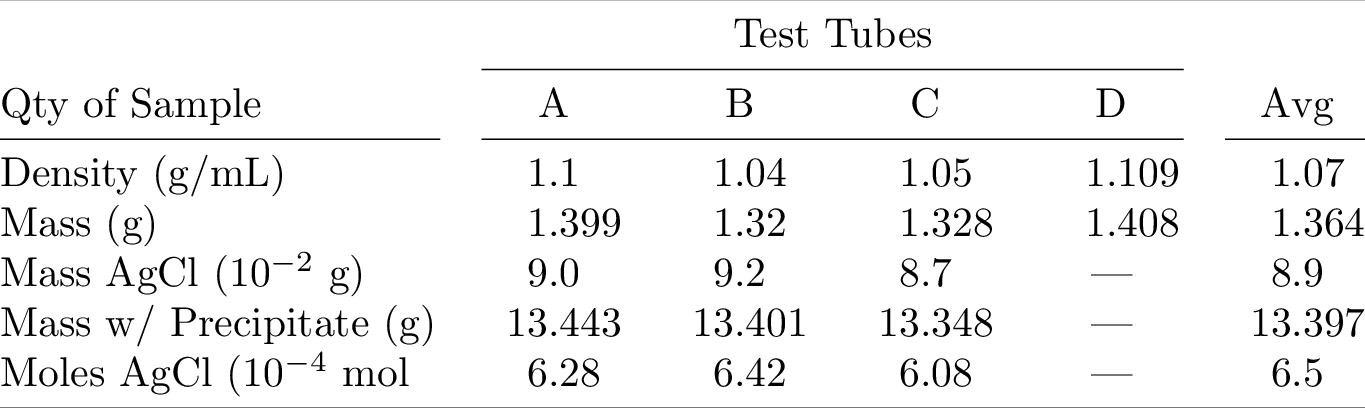
Scientific Table 1
Example from: here
 1import tabx
 2from tabx import DescData, utils, Cmidrule
 3
 4
 5column_names = ["{A}", "{B}", "{C}", "{D}", "{Avg}"]
 6values = [
 7    ["Density (g/mL)", 1.1, 1.04, 1.05, 1.109, 1.07],
 8    ["Mass (g)", 1.399, 1.32, 1.328, 1.408, 1.364],
 9    ["Mass w/ Precipitate (g)", 13.443, 13.401, 13.348, "{---}", 13.397],
10    ["Mass AgCl (\\num{e-2} g)", 9.0, 9.2, 8.7, "{---}", 8.9],
11    ["Moles AgCl (\\num{e-4} mol", 6.28, 6.42, 6.08, "{---}", 6.5],
12]
13desc_datas = DescData.from_values(values, column_names=column_names)
14tab = (
15    tabx.descriptives_table(
16        desc_datas,
17        col_maps=tabx.ColMap(mapping={(1, 4): r"Test Tubes"}),
18        var_name="Qty of Sample",
19        include_midrule=False,
20    )
21    .insert_row(
22        Cmidrule(1, 1, "r") | Cmidrule(2, 5, "rl") | Cmidrule(6, 6, "l"),
23        index=3,
24    )
25    .set_align("l" + 5 * "S")
26)
27file = utils.compile_table(
28    tab.render(),
29    silent=True,
30    name="booktabs1",
31    output_dir=utils.proj_folder().joinpath("figs"),
32)
33_ = utils.pdf_to_png(file)
Compiling the table to PDF and converting it to PNG yields:
Scientific Table 2
Example from: here
 1import tabx
 2from tabx import DescData, utils
 3
 4
 5names = [
 6    r"\texttt{trigmv}",
 7    r"\texttt{trig\_expmv}",
 8    r"\texttt{trig\_block}",
 9    r"\texttt{expleja}",
10]
11desc_datas = [
12    DescData.from_dict(
13        {"variable": names, "values": [11034, 21952, 15883, 11180]},
14        name="$mv$",
15    ),
16    DescData.from_dict(
17        {"variable": names, "values": [1.3e-7, 1.3e-7, 5.2e-8, 8.0e-9]},
18        name="Rel.~err",
19    ),
20    DescData.from_dict(
21        {"variable": names, "values": [3.9, 6.2, 7.1, 4.3]},
22        name="Time",
23    ),
24    DescData.from_dict(
25        {"variable": names, "values": [15846, 31516, 32023, 17348]},
26        name="$mv$",
27    ),
28    DescData.from_dict(
29        {"variable": names, "values": [2.7e-11, 2.7e-11, 1.1e-11, 1.5e-11]},
30        name="Rel.~err",
31    ),
32    DescData.from_dict(
33        {"variable": names, "values": [5.6, 8.8, 14.0, 6.6]},
34        name="Time",
35    ),
36]
37tab = tabx.descriptives_table(
38    desc_datas,
39    col_maps=tabx.ColMap(
40        mapping={
41            (1, 3): r"$\text{tol}=u_{\text{single}}$",
42            (4, 6): r"$\text{tol}=u_{\text{double}}$",
43        }
44    ),
45    var_name="",
46    include_midrule=True,
47)
48file = utils.compile_table(
49    tab.render(),
50    silent=True,
51    name="booktabs2",
52    output_dir=utils.proj_folder().joinpath("figs"),
53)
54_ = utils.pdf_to_png(file)
Compiling the table to PDF and converting it to PNG yields:
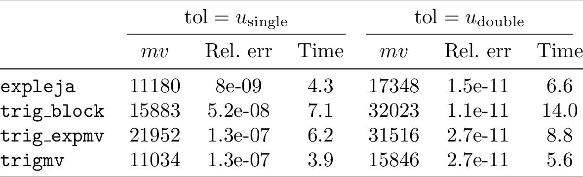
The above is a bit verbose. If you have the data as a list of lists, you
can use DescData.from_values to create the table as follows:
 1column_names = ["$mv$", "Rel.~err", "Time", "$mv$", "Rel.~err", "Time"]
 2values = [
 3    ["\\texttt{trigmv}", 11034, 1.3e-07, 3.9, 15846, 2.7e-11, 5.6],
 4    ["\\texttt{trig\\_expmv}", 21952, 1.3e-07, 6.2, 31516, 2.7e-11, 8.8],
 5    ["\\texttt{trig\\_block}", 15883, 5.2e-08, 7.1, 32023, 1.1e-11, 14.0],
 6    ["\\texttt{expleja}", 11180, 8e-09, 4.3, 17348, 1.5e-11, 6.6],
 7]
 8desc_datas = DescData.from_values(values, column_names=column_names)
 9tab_other = tabx.descriptives_table(
10    desc_datas,
11    col_maps=tabx.ColMap(
12        mapping={
13            (1, 3): r"$\text{tol}=u_{\text{single}}$",
14            (4, 6): r"$\text{tol}=u_{\text{double}}$",
15        }
16    ),
17    var_name="",
18    include_midrule=True,
19)
20print(tab == tab_other)
True
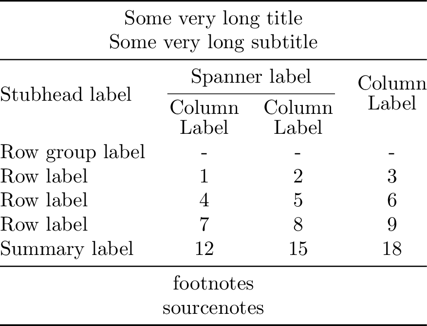
Great Tables
Great Tables table
Construct a table from its components as shown in in Great Tables
 1"""
 2See: https://posit-dev.github.io/great-tables/articles/intro.html
 3"""
 4
 5import tabx
 6
 7from tabx import Table, table, Cmidrule, Midrule
 8from tabx import Cell as C
 9from tabx.table import multicolumn_row, multirow_column
10from tabx.utils import compile_table, render_body_no_rules, pdf_to_png
11
12
13vals = [[j for j in range(i, i + 3)] for i in range(1, 9 + 1, 3)]
14colsums = [sum(col) for col in zip(*vals)]
15table_body = Table.from_values(vals + [colsums])
16stub = table.Column.from_values(
17    ["Row label", "Row label", "Row label", "Summary label"]
18)
19stubhead_label = multirow_column(
20    "Stubhead label",
21    multirow=3,
22    vpos="c",
23    vmove="3pt",
24)
25col_labels1 = (
26    # spanner label
27    C("Spanner label", multicolumn=2)
28    / Cmidrule(1, 2, trim="lr")
29    # column labels
30    / (C(r"\shortstack{Column\\Label}") | C(r"\shortstack{Column\\Label}"))
31)
32col_labels2 = multirow_column(
33    r"\shortstack{Column\\Label}",
34    # "Column label",
35    multirow=3,
36    vpos="c",
37    vmove="3pt",
38)
39col_labels = col_labels1 | col_labels2
40footnotes = multicolumn_row("footnotes", multicolumn=4, colspec="c")
41sourcenotes = multicolumn_row("sourcenotes", multicolumn=4, colspec="c")
42title = multicolumn_row("Some very long title", multicolumn=4, colspec="c")
43subtitle = multicolumn_row("Some very long subtitle", multicolumn=4, colspec="c")
44tab = (
45    (title / subtitle)
46    / Midrule()
47    / (stubhead_label | col_labels)
48    / (C("Row group label") | [C("-"), C("-"), C("-")])
49    / (stub | table_body)
50    / Midrule()
51    / (footnotes / sourcenotes)
52).set_align("lccc")
Compiling the table to PDF and converting it to PNG yields:
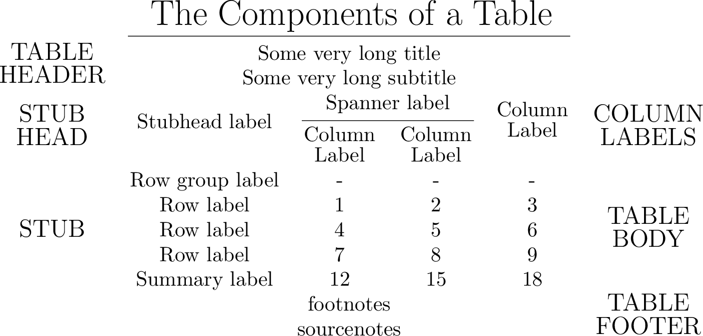
Annotated table
Annotate the table as shown in in Great Tables docs
 1# Remove midrules and annotate the table's components
 2# Midrules will span the annotations; hence we remove them
 3tab = (
 4    (title / subtitle)
 5    / (stubhead_label | col_labels)
 6    / (C("Row group label") | [C("-"), C("-"), C("-")])
 7    / (stub | table_body)
 8    / (footnotes / sourcenotes)
 9).set_align("lccc")
10annotations_left = (
11    multirow_column(r"\large \shortstack{TABLE\\HEADER}", 2, vpos="c")
12    / multirow_column(r"\large \shortstack{STUB\\HEAD}", 3, vpos="c")
13    # add 1 for row group label
14    / multirow_column(r"\large STUB", 4 + 1, vpos="c")
15    / tabx.empty_columns(2, 1)
16)
17annotations_right = (
18    tabx.empty_columns(2, 1)
19    / multirow_column(r"\large \shortstack{COLUMN\\LABELS}", 3, vpos="c")
20    / multirow_column(r"\large \shortstack{TABLE\\BODY}", 4 + 1, vpos="c")
21    / multirow_column(r"\large \shortstack{TABLE\\FOOTER}", 2, vpos="c")
22)
23annotations_top = multicolumn_row(
24    r"\LARGE The Components of a Table", multicolumn=6, colspec="c"
25)
26annotated_tab = (
27    annotations_top / Cmidrule(2, 5) / (annotations_left | tab | annotations_right)
28)
Compiling the table to PDF and converting it to PNG yields:
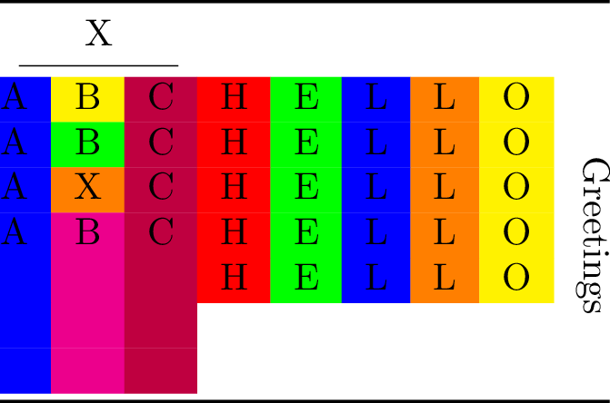
Colored output
 1import tabx
 2from tabx import utils
 3from tabx.utils import colored_column_spec, compile_table, pdf_to_png
 4from tabx import ColoredRow, ColoredCell
 5
 6C = tabx.Cell
 7CC = ColoredCell
 8et = tabx.empty_table
 9CR = ColoredRow
10tab = tabx.Table.from_cells(
11    [
12        [C("A"), CC("B", "yellow"), C("C")],
13        [C("A"), CC("B", "green"), C("C")],
14        [C("A"), CC("X", "orange"), C("C")],
15        [C("A"), C("B"), C("C")],
16    ]
17)
18tab = C("X", multicolumn=3) / tabx.Cmidrule(1, 3) / tab
19tab = (tab / tabx.empty_table(3, 3)).set_align(
20    colored_column_spec("blue", "c")
21    + colored_column_spec("magenta", "c")
22    + colored_column_spec("purple", "r")
23)
24subtab = tabx.Table.from_cells(
25    [
26        [
27            CC("H", "red"),
28            CC("E", "green"),
29            CC("L", "blue"),
30            CC("L", "orange"),
31            CC("O", "yellow"),
32        ]
33        for _ in range(5)
34    ]
35)
36subtab = et(2, 5) / subtab / et(2, 5)
37tab = (
38    tab
39    | subtab
40    | tabx.multirow_column(
41        r"\rotatebox[origin=c]{270}{Greetings}",
42        7,
43        pad_before=2,
44    )
45)
46tab.print()
\begin{tabular}{@{}>{\columncolor{blue}}{c}>{\columncolor{magenta}}{c}>{\columncolor{purple}}{r}cccccc@{}}
  \toprule
  \multicolumn{3}{c}{X} &  &  &  &  &  &  \\
  \cmidrule(lr){1-3}
  A & \cellcolor{yellow}B & C & \cellcolor{red}H & \cellcolor{green}E & \cellcolor{blue}L & \cellcolor{orange}L & \cellcolor{yellow}O & \multirow{7}{*}{\rotatebox[origin=c]{270}{Greetings}} \\
  A & \cellcolor{green}B & C & \cellcolor{red}H & \cellcolor{green}E & \cellcolor{blue}L & \cellcolor{orange}L & \cellcolor{yellow}O &  \\
  A & \cellcolor{orange}X & C & \cellcolor{red}H & \cellcolor{green}E & \cellcolor{blue}L & \cellcolor{orange}L & \cellcolor{yellow}O &  \\
  A & B & C & \cellcolor{red}H & \cellcolor{green}E & \cellcolor{blue}L & \cellcolor{orange}L & \cellcolor{yellow}O &  \\
   &  &  & \cellcolor{red}H & \cellcolor{green}E & \cellcolor{blue}L & \cellcolor{orange}L & \cellcolor{yellow}O &  \\
   &  &  &  &  &  &  &  &  \\
   &  &  &  &  &  &  &  &  \\
  \bottomrule
\end{tabular}
Compiling the table to PDF and converting it to PNG yields:
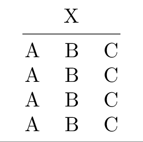
Misc
 1import tabx
 2from tabx import utils
 3from tabx.utils import compile_table, pdf_to_png
 4
 5C = tabx.Cell
 6tab = tabx.Table.from_cells(
 7    [
 8        [C("A"), C("B"), C("C")],
 9        [C("A"), C("B"), C("C")],
10        [C("A"), C("B"), C("C")],
11        [C("A"), C("B"), C("C")],
12    ]
13)
14tab = C("X", multicolumn=3) / tabx.Cmidrule(1, 3) / tab
15tab
Table(nrows=6, ncols=3)
1tab.shape
(6, 3)
1tab.shape
2print(tab.render())  # Rendered table
\begin{tabular}{@{}ccc@{}}
  \toprule
  \multicolumn{3}{c}{X} \\
  \cmidrule(lr){1-3}
  A & B & C \\
  A & B & C \\
  A & B & C \\
  A & B & C \\
  \bottomrule
\end{tabular}
1ce = tabx.empty_columns(6, 1)
2ctab = ce | tab | ce
3ctab.print()
\begin{tabular}{@{}ccccc@{}}
  \toprule
   & \multicolumn{3}{c}{X} &  \\
  \cmidrule(lr){2-4}
   & A & B & C &  \\
   & A & B & C &  \\
   & A & B & C &  \\
   & A & B & C &  \\
  \bottomrule
\end{tabular}
Compiling the table to PDF and converting it to PNG yields:
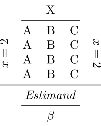
 1rlab = tabx.multirow_column(
 2    r"\rotatebox[origin=c]{90}{$x = 2$}",
 3    4,
 4    pad_before=2,
 5    align="l",
 6)
 7rlab2 = tabx.multirow_column(
 8    r"\rotatebox[origin=c]{270}{$x = 2$}",
 9    4,
10    pad_before=2,
11    align="l",
12)
13tt = (
14    (rlab | tab | rlab2)
15    / tabx.Midrule()
16    / C("Estimand", multicolumn=5, style="italic")
17    / tabx.Cmidrule(2, 4)
18    / C(r"$\beta$", multicolumn=5)
19)
20tt.print()
\begin{tabular}{@{}ccccc@{}}
  \toprule
   & \multicolumn{3}{c}{X} &  \\
  \cmidrule(lr){2-4}
  \multirow{4}{*}{\rotatebox[origin=c]{90}{$x = 2$}} & A & B & C & \multirow{4}{*}{\rotatebox[origin=c]{270}{$x = 2$}} \\
   & A & B & C &  \\
   & A & B & C &  \\
   & A & B & C &  \\
  \midrule
  \multicolumn{5}{c}{\textit{Estimand}} \\
  \cmidrule(lr){2-4}
  \multicolumn{5}{c}{$\beta$} \\
  \bottomrule
\end{tabular}
Compiling the table to PDF and converting it to PNG yields:
Ascii
 1"""
 2ASCII art tables.
 3"""
 4
 5from functools import reduce
 6
 7import pyfiglet
 8
 9import tabx
10from tabx import Cell, utils
11from tabx.utils import render_body_simple
12
13
14def get_lines(c: str):
15    return [c for c in c.splitlines() if c]
16
17
18def parse_c(c: str):
19    if c == "_":
20        return r"\_"
21    if c == "|":
22        return r"\textbar"
23    if c == "\\":
24        return r"\textbackslash"
25    if c == "<":
26        return r"\textless"
27    if c == ">":
28        return r"\textgreater"
29    return c
30
31
32def get_table(s: str):
33    parts = get_lines(s)
34    max_len = max([len(p) for p in parts])
35    rows = []
36    for p in parts:
37        row = []
38        lp = len(p)
39        diff = max_len - lp
40        for c in p:
41            row.append(Cell(value=parse_c(c), style="bold"))
42        for _ in range(diff):  # pad differences
43            row.append(tabx.empty_cell())
44        rows.append(tabx.Row(row))
45    return tabx.Table(rows)
46
47
48p1 = pyfiglet.figlet_format("t")
49p2 = pyfiglet.figlet_format("a")
50p3 = pyfiglet.figlet_format("b")
51p4 = pyfiglet.figlet_format("x")
52
53cols = [
54    get_table(p1),
55    get_table(p2),
56    get_table(p3),
57    get_table(p4),
58]
59
60ec = tabx.empty_columns
61
62tab = get_table(p1) | get_table(p2) | get_table(p3) | get_table(p4)
63file = utils.compile_table(
64    tab.render(),
65    silent=True,
66    output_dir=utils.proj_folder().joinpath("figs"),
67    name="ascii1",
68)
69_ = utils.pdf_to_png(file)
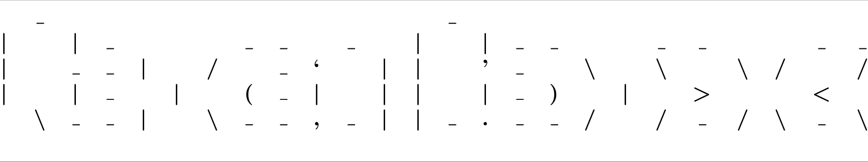
 1words = []
 2for word in ["LaTeX", "tables", "in", "Python"]:
 3    word_cols = []
 4    for c in word:
 5        word_cols.append(get_table(pyfiglet.figlet_format(c)))
 6    words.append(reduce(lambda x1, x2: x1 | x2, word_cols))
 7extra = (words[0] | ec(6, 1) | words[1]) / (
 8    ec(6, 7) | words[2] | ec(6, 3) | words[3] | ec(6, 7)
 9)
10top = ec(6, 21) | tab | ec(6, 21)
11
12r = file = utils.compile_table(
13    (top / extra).render(render_body_simple),
14    silent=True,
15    output_dir=utils.proj_folder().joinpath("figs"),
16    name="ascii2",
17)
18_ = utils.pdf_to_png(file)

CLI
tabx --help
usage: tabx [-h] {compile,check} ...

tabx CLI

positional arguments:
  {compile,check}
    compile        Compile a LaTeX table to PDF.
    check          Check if LaTeX compilers are available.

options:
  -h, --help       show this help message and exit
tabx compile --help
usage: tabx compile [-h] (--file FILE | --stdin)
                    [--command {pdflatex,lualatex,xelatex}]
                    [--output-dir OUTPUT_DIR] [--name NAME] [--silent]
                    [--extra-preamble EXTRA_PREAMBLE]

options:
  -h, --help            show this help message and exit
  --file FILE           Path to file containing LaTeX table.
  --stdin               Read LaTeX table from stdin.
  --command {pdflatex,lualatex,xelatex}
                        LaTeX engine to use (default: pdflatex).
  --output-dir OUTPUT_DIR
                        Directory for output PDF (default: cwd).
  --name NAME           Base name for output file (default: table).
  --silent              Suppress LaTeX output.
  --extra-preamble EXTRA_PREAMBLE
                        Extra LaTeX preamble content.
tabx check --help
usage: tabx check [-h]

options:
  -h, --help  show this help message and exit
Compile table
python -c 'import tabx
tab = tabx.Table.from_values([[1, 2, 3], [4, 5, 6], [7, 8, 9]])
tabx.save_table(tab, "/tmp/table.tex")
'
cat /tmp/table.tex
\begin{tabular}{@{}ccc@{}}
  \toprule
  1 & 2 & 3 \\
  4 & 5 & 6 \\
  7 & 8 & 9 \\
  \bottomrule
\end{tabular}
tabx compile --file /tmp/table.tex --output-dir /tmp/ --silent
Compiled PDF saved to: /tmp/table.pdf
or from stdin
tabx compile --stdin --output-dir /tmp/ --silent < /tmp/table.tex
Compiled PDF saved to: /tmp/table.pdf
Check latex commands available
tabx check
pdflatex: found at /usr/bin/pdflatex
lualatex: found at /usr/bin/lualatex
xelatex: found at /usr/bin/xelatex
Development
git clone git@github.com:jsr-p/tabx.git
cd tabx
uv venv
uv sync --all-extras
Contributions
Contributions are welcome!
Misc.
Alternatives
The alternatives below are great but didn’t suit my needs fiddling with
multicolumn cells, multirow cells, cmidrules etc. and using the
tabular environment in LaTeX.
Why not tabularray?
The reason for using tabular + booktabs instead of tabularray is that tabularray is too slow when compiling. Also, tabular + booktabs is all you need.