Axler example

Example 6.63 from Axler’s Linear Algebra Done Right 🙏

The problem

Goal: compute an approximation to the sine function that improves upon the Taylor Polynomial approximation from calculus.

• Let C[-\pi, \pi] denote the real inner product space of continuous real-valued functions on [-\pi, \pi] with inner product \langle f, g \rangle = \int_{-\pi}^{\pi} fg.

• Let v \in C[-\pi, \pi] be the function v(x) = \sin x

• Let U denote the subspace \mathcal{P}_{5}(\mathbb{R}) \subseteq C[-\pi, \pi] (the space of polynomials of degree at most 5 with real coefficients)

• The goal is to choose u \in U such that \Vert v - u \Vert is as small as possible where

\begin{align*} \Vert v - u \Vert = \int_{-\pi}^{\pi} \vert \sin x - u(x) \vert^{2} dx. \end{align*}

• The solution is given by the orthogonal projection of v(x) = \sin x onto U = \mathcal{P}_{5}(\mathbb{R})

Approach:

• Have standard basis of \mathcal{P}_{5}(\mathbb{R})

\begin{align*} (v_{1}, v_{2}, v_{3}, v_{4}, v_{5}, v_{6}) = (1, x, x^{2}, x^{3}, x^{4}, x^{5}). \end{align*}

• Compute orthonormal basis of \mathcal{P}_{5}(\mathbb{R}) by applying the Gram-Schmidt procedure to the basis above.

• The kth vector of the orthonormal basis is computed as:

\begin{align*} f_{k} & = v_{k} - \frac{\langle v_{k}, f_{1} \rangle}{\Vert f_{1} \Vert^{2}} f_{1} - \cdots - \frac{\langle v_{k}, f_{k - 1} \rangle}{\Vert f_{k - 1} \Vert^{2}} f_{k - 1} \\ e_{k} & = \frac{f_{k}}{\Vert f_{k} \Vert}. \end{align*}

• Compute the orthogonal projection of v(x) = \sin x onto \mathcal{P}_{5}(\mathbb{R}) by using the orthonormal basis found above and the formula:

\begin{align*} P_{U}v = \langle v, e_{1} \rangle e_{1} + \cdots + \langle v, e_{m} \rangle e_{m}. \end{align*}

Code

See the repo for the full code.

We’ll have to do two things:

1. Compute the orthonormal basis of \mathcal{P}_{5}(\mathbb{R}) using the Gram-Schmidt procedure on the standard basis (1, x, x^{2}, x^{3}, x^{4}, x^{5})

2. Compute the orthogonal projection of the function v(x) = \sin x using the orthonormal basis computed in the first step and the decomposition formula

The hard part is computing the inner products (and norms). Recall that the inner product in this example is an integral over the interval [- \pi, \pi]. Fortunately, with the great Python library sympy, we can compute such an integral symbolically with relative ease.

The function comp_int below computes the integral \int_{-\pi}^{\pi} f(x) dx:

import sympy as sp
from sympy import Symbol, integrate, pi, sqrt

# Polynomial basis
x = Symbol("x")
v1 = sp.Integer("1")
v2 = x
v3 = x**2
v4 = x**3
v5 = x**4
v6 = x**5

v = sp.sin(x)  # The function we approximate on [-π, π]


def comp_int(f):
    """Compute integral of f on [-pi, pi]"""
    return integrate(f, (x, -pi, pi))

The inner product between two functions f and g can then be computed by applying comp_int to the product of the two functions f \cdot g:

def inp(f, g):
    return comp_int(f * g)

The orthonormal basis is computed using the function:

GSVec = namedtuple(
    "GSVec",
    ["f", "norm", "norm_sq", "e"],
)
GSVecs: TypeAlias = dict[int, GSVec]


def gram_schmidt(basis: dict[int, sp.Expr]) -> GSVecs:
    gs_vecs: GSVecs = dict()
    f1 = basis[1]
    ns_f1 = norm_sq(f1)
    n_f1 = sqrt(ns_f1)
    e1 = f1 / n_f1
    gs_vecs[1] = GSVec(f1, n_f1, ns_f1, e1)
    for k in range(2, 6 + 1):
        v_k = basis[k]
        f_k = gs_step(v_k, list(gs_vecs.values()))
        ns_fk = norm_sq(f_k)
        n_fk = sqrt(ns_fk)
        gs_vecs[k] = GSVec(f_k, n_fk, ns_fk, f_k / n_fk)
    return gs_vecs

The final step is then to compute the orthogonal projection of the function using the orthonormal basis:

def projection_gs(v, gs_vecs: GSVecs):
    r"""Projects v onto the subspace spanned by the orthonormal basis"""
    return sum([inp(v, gs.e) * gs.e for gs in gs_vecs.values()])

See the full script here

def main():
    # Compute orthonormal basis
    basis = dict(zip(range(1, 6 + 1), [v1, v2, v3, v4, v5, v6]))
    gs_vecs = gram_schmidt(basis)
    # Compute the orthogonal projection of v onto the subspace
    proj = projection_gs(v, gs_vecs)
    # Print the projection
    print(f"\nProjection exact (latex):\n\t{sp.latex(proj)}")

Result

The projection of v(x) = \sin x onto the subspace \mathcal{P}_{5}(\mathbb{R}) is given by the exact formula: \begin{aligned} & P_U v = \frac{3 x}{\pi^{2}} + \frac{5 \sqrt{14} \left(x^{3} - \frac{3 \pi^{2} x}{5}\right) \left(- \frac{5 \sqrt{14} \left(- \frac{2 \pi^{3}}{5} + 6 \pi\right)}{4 \pi^{\frac{7}{2}}} + \frac{5 \sqrt{14} \left(- 6 \pi + \frac{2 \pi^{3}}{5}\right)}{4 \pi^{\frac{7}{2}}}\right)}{4 \pi^{\frac{7}{2}}} \\ & + \frac{1}{16 \pi^{\frac{11}{2}}} \times 63 \sqrt{22} \left(- \frac{63 \sqrt{22} \left(- 120 \pi - \frac{8 \pi^{5}}{63} + \frac{40 \pi^{3}}{3}\right)}{16 \pi^{\frac{11}{2}}} + \frac{63 \sqrt{22} \left(- \frac{40 \pi^{3}}{3} + \frac{8 \pi^{5}}{63} + 120 \pi\right)}{16 \pi^{\frac{11}{2}}}\right) \\ & \times \left(x^{5} - \frac{3 \pi^{4} x}{7} - \frac{10 \pi^{2} \left(x^{3} - \frac{3 \pi^{2} x}{5}\right)}{9}\right) \frac{}{} \end{aligned}

This formula is the output of sp.latex(proj), thanks sympy!

This is approximately equal to \begin{aligned} P_U v \approx 0.987862135574673 \cdot x - 0.155271410633428 \cdot x^{3} + 0.00564311797634678 \cdot x^{5} \end{aligned}

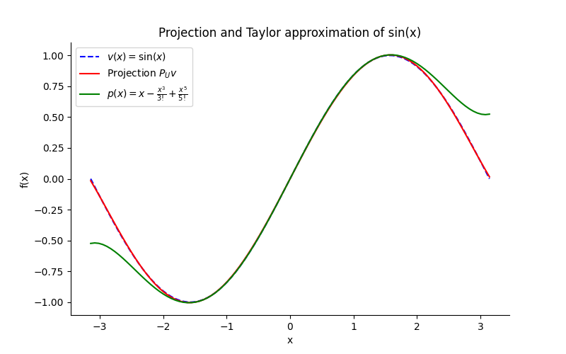
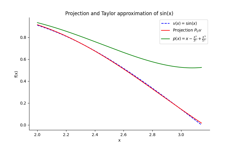
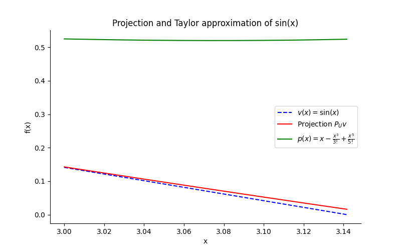
Plots

The plots below compare the sine function with the found orthogonal projection and the classical fifth-order Taylor polynomial (approximation).

And seen from the plots, the projection is much closer to the sine function than the Taylor polynomial. True mathmagic!